System and surroundings — Choose the reacting chemicals as the system and identify the surroundings exchanging energy with it. At constant pressure, the enthalpy change corresponds to heat transferred to the system under the usual chemistry assumptions. A temperature rise in the surroundings therefore commonly indicates a negative reaction enthalpy, not a positive one.
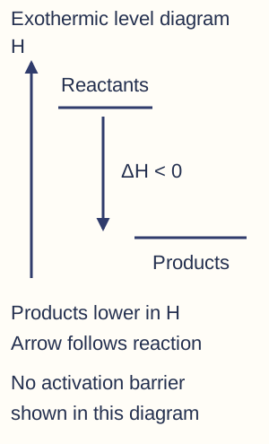
Exothermic and endothermic — An exothermic reaction transfers energy from the system and has ΔH < 0; an endothermic reaction absorbs energy and has ΔH > 0. On an enthalpy level diagram, products lie below reactants for an exothermic reaction and above for an endothermic one. Label the arrow in the reaction direction and attach the correct sign.Schematic enthalpy levels for an exothermic reaction. The downward reaction arrow gives a negative enthalpy change. This level diagram does not depict an activation barrier; horizontal placement is for clarity and is not time or a measured reaction coordinate.
Energy levels versus profiles — An enthalpy level diagram compares initial and final states. A reaction profile additionally represents an activation barrier along a reaction pathway. Neither horizontal axis is automatically time. A catalyst changes the pathway and activation barrier but not the reactant–product enthalpy difference under the same conditions.
Standard-state care — The standard pressure is 100 kPa and a temperature must be specified, commonly 298 K. A substance's standard state is its relevant physical form under the specified conditions. Include state symbols: H2O(l) and H2O(g) do not have the same formation enthalpy. Standard does not mean zero degrees Celsius or one mole of every reactant in every definition.
Standard reaction enthalpy — The standard enthalpy change of reaction is the enthalpy change for the reaction as written, with reactants and products in their standard states at the specified temperature. Changing the balanced equation's scale changes its associated reaction enthalpy; reversing the reaction changes its sign.
Standard formation enthalpy — The standard enthalpy change of formation is for forming one mole of a compound from its constituent elements in their standard states under standard conditions. For water(l), H2(g) + 1/2 O2(g) → H2O(l) forms exactly one mole. An element in its reference standard state has zero standard formation enthalpy by convention; isolated gaseous atoms need not.
Standard combustion enthalpy — The standard enthalpy change of combustion is for complete combustion of one mole of a substance in oxygen under standard conditions, with all specified species in standard states. CH4(g) + 2O2(g) → CO2(g) + 2H2O(l) is a suitable equation. Incomplete production of CO or soot does not measure that complete-combustion change directly.
Standard neutralisation enthalpy — The standard enthalpy change of neutralisation is the change when acid and base react to form one mole of water under standard conditions. Strong aqueous acid and hydroxide largely share H+ + OH− → H2O, giving a similar value near −57 kJ mol−1 under comparable conditions. Count moles of water formed, not whichever solution volume is largest.
Weak-acid comparison — A weak acid is only partly dissociated, so neutralisation includes the energetic consequences of further ionisation as H+ is consumed. Values can differ from strong-acid neutralisation. Do not claim every weak acid must have one identical extra energy cost; actual ionisation enthalpy and conditions matter alongside concentration and heat-loss effects.
Calorimetry and experimental evaluation
Temperature and heat — Use q = mcΔT for the chosen heated or cooled material, with mass m, specific heat capacity c and temperature change ΔT. If c is in J g−1 K−1 and m in grams, q is in joules. A temperature interval of one kelvin equals one Celsius degree, but absolute temperature in thermodynamic equations must be kelvin.
Solution assumptions — For dilute aqueous solutions a calculation may approximate density as 1.00 g cm−3 and c as 4.18 J g−1 K−1. Use the combined solution mass when appropriate, not only the mass of dissolved solute. These are assumptions to evaluate, not exact constants for every acid, salt, solvent or concentrated mixture.
Calorimeter and reaction signs — The calculated heat gained by the solution is positive if its temperature rises. For an approximately insulated setup, the reaction loses that heat: qreaction ≈ −qsolution. If calorimeter heat capacity is known, include its heat term as well. Attach the sign only after identifying whose heat change was calculated.
Worked neutralisation — Mix 25.0 cm3 of 1.00 mol dm−3 HCl with 25.0 cm3 of 1.00 mol dm−3 NaOH. If the 50.0 g solution rises by 6.50 K using c = 4.18, qsolution = 1358.5 J. Water formed is 0.0250 mol, so ΔH ≈ −1358.5/0.0250 = −54.3 kJ mol−1 after converting J to kJ.
Limiting reagent and normalization — If acid and base amounts are unequal, use the limiting stoichiometric amount to calculate water formed. A diprotic acid can donate two protons per molecule and therefore provide two proton equivalents under the stated complete-neutralisation model. Dividing measured heat by total solution volume or total combined reagent moles does not produce a valid molar reaction enthalpy.
Insulated-container technique — Use an appropriate insulated container with a lid, controlled starting temperatures, measured amounts and mixing. Record temperature against time before and after mixing using an approved method. Account for probe response, incomplete reaction and transfer heat; merely adding more decimal places to a thermometer does not remove systematic heat exchange.
Extrapolated temperature change — When heat exchange affects a cooling trace, extrapolate an appropriate post-reaction trend back to the mixing time and compare it with the initial-temperature trend there. Show the mixing time, fitted regions and temperature difference. Extrapolation depends on the model and timing; it is not permission to choose a line yielding the expected answer.
Combustion calorimetry — Heat a known mass of water using a measured loss of fuel mass and calculate heat transferred to the water. Divide by the fuel amount burned, with the reaction sign. Record conditions and account for heat absorbed by the container where relevant; the mass lost from a burner is not automatically the mass completely combusted.
Worked combustion estimate — A burner loses 0.460 g ethanol, equivalent to 0.0100 mol using M = 46.0. Heating 100 g water by 20.0 K transfers 8360 J using c = 4.18. The simple experimental estimate is ΔHc ≈ −836 kJ mol−1. This illustrative value is not a tabulated standard value or evidence that all combustion heat reached the water.
Evaluating heat-loss bias — Heat escaping to air or warming unaccounted apparatus usually reduces the measured water temperature rise for an exothermic reaction, making the inferred ΔH less negative. Incomplete combustion and fuel evaporation can have related effects for a burner. Explain the causal chain from the fault to measured variables and calculated result rather than saying human error.
Uncertainty and design — For q = mcΔT, estimate relevant mass, temperature and amount uncertainties using the required convention; a small temperature difference can have a large percentage uncertainty. Larger controlled temperature changes, suitable insulation and better timing can improve evidence, but changes must respect safe concentrations, apparatus and reaction rates.
Hess cycles and mean bond enthalpies
Hess's law — Enthalpy is a state function: for the same initial and final states, the total enthalpy change is independent of the route. Construct alternative routes with fully balanced species and states. The law does not say every intermediate step is physically convenient or that reaction speed is independent of pathway.
Formation-enthalpy calculation — Use ΔrH° = ΣνΔfH°(products) − ΣνΔfH°(reactants), with balanced coefficients ν. The symbol Σ means add all the relevant terms, multiplying each substance's value by its equation coefficient ν. For CH4 + 2O2 → CO2 + 2H2O(l), illustrative formation values −75, 0, −394 and −286 kJ mol−1 give (−394 + 2 × −286) − (−75) = −891 kJ mol−1. Check the water state and equation scale.
Combustion-enthalpy route — If reactants and products can each burn to the same final species, equate the two routes. For A → B, ΔHreaction = total combustion enthalpy of A − total combustion enthalpy of B after balancing all materials. This subtraction order differs from the usual products-minus-reactants formation formula because the route arrows point toward common combustion products.
Reversing and scaling steps — For an illustrative A → C change of −120 kJ mol−1 and B → C change of −80 kJ mol−1, A → B is −40 kJ mol−1. Reverse the B → C arrow to obtain +80, then add to −120. If an equation is doubled, double its heat contribution; if it is reversed, reverse the sign.
Indirect enthalpy measurement — A reaction that cannot be measured directly can be inferred by measuring two routes to a common final state, such as dissolving an anhydrous salt and its hydrate. Include the correct number of waters in the equations so the overall initial and final states match. Different final solution concentrations can undermine a simplistic comparison.
Core Practical 8 evidence — Measure the prescribed reaction changes using suitable calorimetry, calculate each molar enthalpy and construct the actual Hess cycle with directions and coefficients. Evaluate insulation, dissolution completeness, material hydration and final-state assumptions. A correct cycle from supplied data does not certify that a learner performed the measurements competently.
Bond enthalpy — A bond dissociation enthalpy is for breaking a specified mole of bonds in gaseous species by homolytic cleavage, where each bonded atom receives one of the shared electrons. Bond breaking requires energy and bond formation releases energy. A mean bond enthalpy averages a bond type over different suitable gaseous environments, so it cannot perfectly represent every bond bearing that label.
Using bond enthalpies — Estimate ΔH = Σ bond enthalpies broken − Σ bond enthalpies formed for a gas-phase reaction. Count all bonds in the balanced equation, cancelling unchanged ones only when appropriate. Liquid or solid species need additional state-change terms if the target reaction is not entirely gaseous.
Worked bond estimate — For H2(g) + Cl2(g) → 2HCl(g), illustrative H–H = 436, Cl–Cl = 243 and H–Cl = 431 kJ mol−1 give ΔH ≈ 436 + 243 − 2 × 431 = −183 kJ mol−1. Forming two H–Cl bonds is essential; counting only one reverses the intended energy accounting.
Finding an unknown bond value — Rearrange the same broken-minus-formed expression for an unknown bond enthalpy. If the reaction above has ΔH = −184 using H–H = 436 and Cl–Cl = 243, then 2D(H–Cl) = 436 + 243 + 184, giving 431.5 kJ mol−1. The coefficient belongs to the number of bonds formed, not to a change in their units.
Mean-bond limitations — Bond strengths vary with molecular environment, and average values give estimates. Additional errors arise from wrong states, incorrect structures or missed multiple bonds. An average estimate differing from a precise experimental ΔH does not disprove Hess's law, which concerns exact state changes rather than approximate input values.
Lattice, atomisation and electron-affinity cycles
Lattice formation convention — Here lattice energy is the enthalpy change when one mole of an ionic solid forms from its gaseous ions, for example Na+(g) + Cl−(g) → NaCl(s). It is negative for the lattice formation process. Some sources quote lattice dissociation instead, with the opposite sign, so write the process rather than relying on the word lattice alone.
Atomisation — The enthalpy change of atomisation forms one mole of gaseous atoms from an element in its stated standard form. For chlorine, 1/2 Cl2(g) → Cl(g) uses half the Cl–Cl dissociation enthalpy; for sodium, Na(s) → Na(g) includes conversion from the metal. Producing a mole of molecules is not atomisation.
Electron affinities — The first electron affinity is the change for X(g) + e− → X−(g), one mole of gaseous negative ions formed from gaseous atoms. It is often exothermic. Adding a second electron to an already negative ion is endothermic because of repulsion; do not assign both electron-affinity steps the first step's sign.
Born–Haber construction — Connect the elements in standard states to the ionic solid directly by formation enthalpy and indirectly by atomisation, ionisation, electron affinity and lattice formation. Every gas-ion step must produce the correct charge and number of ions. For MgCl2, use two chlorine atomisation amounts and two first electron affinities, plus both magnesium ionisation energies.
Worked sodium chloride cycle — Using illustrative kJ mol−1 values ΔfH = −411, Na atomisation +108, chlorine atomisation +121, Na first ionisation +496 and chlorine first electron affinity −349, −411 = 108 + 121 + 496 − 349 + ΔlatticeH. Therefore ΔlatticeH = −787 kJ mol−1 for formation from gaseous ions.Balanced sodium chloride Born–Haber route using illustrative values in kJ mol−1. Atomisation +229, ionisation +496, electron affinity −349 and lattice formation −787 sum to direct formation −411. Vertical positions show the sequence of transformations only, not relative energy levels; signs and values give the actual energy changes.
Oxide-cycle electron accounting — For MgO, the oxygen atom gains two electrons through separate first and second electron-affinity steps, while magnesium loses two through successive ionisation steps. The large positive second electron affinity must be included. A stable solid can form overall because other favourable terms, especially lattice formation, outweigh costly gas-phase ion production.
Charge and separation — Greater ionic charges and smaller separation generally increase electrostatic attraction, making lattice formation more exothermic for comparable structures. The trend is not determined by cation radius alone: charge, both ions' sizes and crystal arrangement matter. Compare the magnitudes and the stated sign convention carefully.
Polarising ions — A small, highly charged cation has strong polarising power; a large anion, especially with more negative charge, can be more readily distorted. Distortion shifts electron density away from an ideal separate spherical-ion picture and introduces covalent character. Polarising power of the cation is not the same property as polarisability of the anion.
Experimental versus ionic-model lattice values — A Born–Haber value inferred from thermochemical data can be compared with an ideal electrostatic ionic-model prediction. Close agreement supports a largely ionic description; a more exothermic experimental formation value can indicate extra stabilisation associated with covalent character. Compare the same convention and acknowledge model assumptions rather than treating a percentage difference as an exact bond-type percentage.
Solution and hydration energetics
Enthalpy of solution — The enthalpy change of solution is the change when one mole of solute dissolves under the specified conditions, usually with sufficient solvent to approach the reference dilute state. Write the actual initial solid and final aqueous ions. An anhydrous salt and its hydrate can have different solution enthalpies because their initial states differ.
Enthalpy of hydration — The enthalpy change of hydration forms one mole of aqueous ions from one mole of gaseous ions under the specified conditions, for example Mg2+(g) → Mg2+(aq). Ion–dipole attractions make hydration generally exothermic. Aqueous ions are solvated, meaning surrounded by interacting solvent molecules (water here), not isolated gaseous ions merely placed in an empty container.
Solution cycle — To dissolve an ionic solid, reverse lattice formation to separate gaseous ions, then hydrate them. Hence ΔsolH = −Δlattice,formationH + sum of hydration enthalpies with correct coefficients. If lattice formation is −780 and combined hydration −760 kJ mol−1, solution enthalpy is +20 kJ mol−1, not −1540.
Hydration trends — Higher charge and smaller ionic radius generally give stronger ion–water attraction and more negative hydration enthalpy. These changes can also affect lattice energy, so one term alone does not establish the solution enthalpy or solubility. Entropy is also relevant to whether dissolution is thermodynamically favourable.
Measuring solution enthalpy — Dissolve a known amount in a measured solvent quantity using suitable calorimetry and allow for the resulting solution mass and heat capacity. A fall in solution temperature indicates an endothermic dissolution in the simple insulated model. Check complete dissolution and the salt's hydration state before assigning a molar value.
Entropy of system and surroundings
Why enthalpy is insufficient — Some endothermic processes occur without continuous external work, including suitable salt dissolution. Feasibility therefore cannot be decided from the sign of ΔH alone. Consider energy dispersal and the number of accessible microscopic arrangements of the system and surroundings together, often described at this level as disorder.
State and particle trends — Molar entropy is entropy per mole of substance. It describes energy dispersal and the number of accessible microscopic arrangements, rather than simply how untidy a substance looks. A gas generally has greater molar entropy than its corresponding liquid, and a liquid greater than its solid, under comparable conditions. An increase in gas amount often gives positive system entropy change. These are useful qualitative guides, not substitutes for supplied molar entropy values in a numerical calculation.
Dissolution qualification — Dispersing ions from a crystal can increase positional arrangements, but hydration can order surrounding water. Overall system entropy of dissolution can therefore be positive or negative depending on the actual ions and states. Do not assume every dissolution must increase entropy solely because a solid vanishes.
Calculating system entropy — Use ΔSsystem = ΣνS°(products) − ΣνS°(reactants), with balanced coefficients and units commonly J mol−1 K−1. For illustrative A(g) → 2B(g) with entropies 100 and 80, ΔSsystem = 2 × 80 − 100 = +60 J mol−1 K−1. Standard molar entropy of an element at 298 K is not set to zero like its formation enthalpy.
Surroundings entropy — For heat exchanged with surroundings at temperature T, use ΔSsurroundings = −ΔH/T in the stated constant-pressure approximation. Express ΔH in joules if entropy is required in J mol−1 K−1, and use absolute T in kelvin. An exothermic reaction gives positive surroundings entropy; an endothermic one gives negative.
Total entropy and feasibility — ΔStotal = ΔSsystem + ΔSsurroundings. A positive total change indicates the thermodynamically favourable direction under the specified conditions; at equilibrium there is no positive net driving change. The system alone may become more ordered provided the surroundings gain enough entropy.
Worked total-entropy example — If ΔH = −30.0 kJ mol−1 and ΔSsystem = −50.0 J mol−1 K−1 at 300 K, surroundings entropy is +100 J mol−1 K−1. Total entropy is +50.0 J mol−1 K−1, so the written process is thermodynamically favourable under these assumptions despite the negative system entropy change.
Interpreting contrasting reactions — Magnesium combustion is strongly exothermic even though consuming oxygen gas can reduce system entropy. Dissolving ammonium nitrate can be endothermic yet feasible because favourable system entropy outweighs the surroundings loss. Use actual equations and states before comparing; do not infer the total merely from a temperature change.
Gas-producing endothermic examples — Ethanoic acid reacting with ammonium carbonate can release gas, and the barium hydroxide octahydrate–ammonium chloride demonstration produces ammonia, water and barium chloride while cooling. Product dispersal can favour system entropy. These are explanation examples requiring an approved supervised method, not directions to handle barium compounds or ammonia independently.
Gibbs energy, temperature and equilibrium
Gibbs criterion — At constant temperature and pressure, the Gibbs free-energy change ΔG = ΔH − TΔSsystem links enthalpy and system entropy. ΔG combines the energetic and entropy contributions to the reaction's driving tendency under these conditions. A negative ΔG supports feasibility in the written direction under the specified conditions. Keep all energy units consistent; the entropy term must not accidentally be a thousand times too large or small.
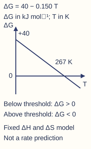
Worked Gibbs calculation — With ΔH = +40.0 kJ mol−1 and ΔSsystem = +150 J mol−1 K−1, at 298 K use +0.150 kJ mol−1 K−1: ΔG = 40.0 − 298 × 0.150 = −4.70 kJ mol−1. The endothermic reaction is thermodynamically favourable at this temperature in the model.
Temperature threshold — Set ΔG = 0 to obtain T = ΔH/ΔSsystem when the changes can be treated as approximately constant over the range. In the previous example T ≈ 267 K, so the positive-ΔH, positive-ΔS reaction becomes favourable above that threshold. Check signs and phases before extending the result to a real temperature range.Illustrative linear fixed-data model for ΔH = +40 kJ mol−1 and ΔSsystem = +0.150 kJ mol−1 K−1. The line crosses zero at about 267 K: higher temperature favours the written reaction in this model. Axis positions and drawn line are schematic; phase and data changes limit real extrapolation.
Sign combinations — Negative ΔH with positive ΔS favours the reaction at all positive temperatures in the simple fixed-value model; positive ΔH with negative ΔS does not. If both are negative, low temperature is favoured; if both positive, high temperature is favoured. Actual phase changes and temperature dependence limit an unlimited extrapolation.
Gibbs energy and equilibrium constant — Here ln means the natural logarithm, with base e, and exp reverses it. For example, ln(e²) = 2. Use ΔG° = −RT ln K for the standard Gibbs change and thermodynamic equilibrium constant at that temperature. R = 8.31 J mol−1 K−1 requires ΔG° in joules. K > 1 gives ΔG° < 0; K = 1 gives zero. This standard change is distinct from the actual reaction Gibbs change, which is zero at equilibrium whatever K.
Worked equilibrium calculation — For ΔG° = −10.0 kJ mol−1 at 300 K, ln K = 10000/(8.31 × 300) ≈ 4.01 and K ≈ 55.2. Use the natural exponential rather than base-ten power. A large K favours products at equilibrium but does not itself give a reaction time or remove the need for a mass-balance calculation.
Relating the criteria — Under the matching assumptions, ΔG = −TΔStotal, so negative Gibbs change and positive total entropy express the same direction of thermodynamic favourability. Do not substitute total entropy into ΔG = ΔH − TΔSsystem; that would count the enthalpy-related surroundings contribution twice.
Kinetic inhibition — A negative ΔG can coexist with a very slow observable reaction because an activation barrier limits successful reaction events. A catalyst may make the pathway faster while leaving ΔG°, K and the equilibrium composition unchanged at fixed temperature. Distinguish thermodynamic feasibility, kinetic rate and practical process choice in a complete conclusion.
Test yourself
50 questions · Random sets of 10. These quick checks support revision; practise longer explanations and justified judgements too.
 Mr Kidman's Classroom