K5CS4 · Abstraction, languages and computation · AQA A-level Computer Science (VB.NET)

Revise the key ideas

Logic problems, algorithms and evidence

Constraints and logical solutions — Translate a logic problem into explicit variables, allowed values and constraints before guessing a solution. If exactly one of P and Q must be true, P Or Q alone is insufficient because both true would also satisfy it; Xor expresses the intended two-input condition. Check every stated constraint, including exclusions and exactly-one requirements.
Systematic reasoning — For a small finite problem, enumerate candidate assignments or use deductions to rule them out. A traceable table can show why a candidate fails and whether one, several or no solutions remain. Finding one valid arrangement does not establish uniqueness unless all alternatives are excluded or an appropriate argument proves it.
Finite algorithm and supported inputs — An algorithm in this course is a precise, finite method that terminates for its defined supported inputs and accomplishes the stated task. A program can implement that method, while a reactive program may deliberately continue waiting for events. An arbitrary program text is not automatically a correct terminating algorithm merely because it contains a loop condition.
Pseudocode and translation — Express the solution using sequence, assignment, selection and iteration with declared meaning for indices, bounds and operators. Translate those operations into VB.NET while accounting for language conventions such as inclusive For bounds, zero-based arrays and integer division. Pseudocode is a communication form, not executable proof independent of its defined semantics, the meanings assigned to its operations and statements.
Trace and justify — Hand-trace changing state, then explain why the process preserves required properties and progresses toward completion. For a running sum, a useful invariant is that total equals the sum of values already processed; incrementing the index eventually exhausts a finite input. The invariant connects the trace to the promised result rather than merely showing that values change.
Testing and feedback — Use typical, boundary and invalid data with independently expected outcomes, and test integration as well as components. User feedback can reveal misunderstood requirements or unusable output even when arithmetic is correct. Tests and feedback support an argument, but a few successful runs do not prove all-input correctness or establish an asymptotic complexity bound by themselves.

Abstraction, hiding and automation

Representational abstraction — A model retains details relevant to a purpose and omits unnecessary detail. A route graph can retain permitted connections and travel costs while omitting a station's paint colour. What is unnecessary depends on the question: omitting step-free access is inappropriate if the task is to plan an accessible route.
Generalisation and categorisation — Generalisation groups common characteristics into a broader category, creating an is-a-kind-of hierarchy. Circle and Rectangle can be categories of Shape with shared area-related behaviour. This abstracts common promises without asserting every subclass has identical representation or that any two nouns justify an inheritance relationship.
Information hiding — Hide internal details that clients do not need to use an abstraction correctly, exposing a stable interface and relevant constraints. A stack client calls Push and Pop without altering its array indices directly. This supports change and reasoning; information hiding is not automatically encryption, confidentiality or a guarantee of protection against a malicious actor.
Procedural abstraction — A procedure captures a computational pattern by replacing particular actual values with parameters. Rather than rewriting the same steps to total three different lists, define a routine receiving a list and following one documented method. The abstraction identifies reusable computation while retaining the idea of a particular procedure for carrying it out.
Functional abstraction — Functional abstraction goes further by describing the input-to-result mapping while disregarding the particular computation method. A square function maps x to x² whether its implementation multiplies x by itself or uses another equivalent method. This mathematical idea is not merely the fact that a language declaration happens to use the keyword Function.
Data abstraction — A data abstraction separates how a compound object is used from how it is represented. The same stack contract can be realised by an array/top index or linked nodes. Clients should depend on the defined operations and failure behaviour, not an assumption that the top item is stored at a particular memory address.
Problem abstraction and reduction — Remove or transform irrelevant details so the problem becomes an instance of one already understood. A least-cost communication problem can reduce to a nonnegative weighted shortest-path problem after defining vertices, edges and additive costs. The reduction is valid only if the retained structure preserves the original objective and constraints.
Decomposition — Break a problem into subproblems accomplishing identifiable tasks, possibly subdividing them further. Separate loading records, validating values, calculating results and presenting output through explicit interfaces. Decomposition is about manageable coherent responsibilities, not merely giving each arbitrary block of lines its own name.
Composition of procedures and data — Combine simpler routines into a larger operation and simpler data objects into a compound model. A report routine can compose validation, summarising and formatting; a tree combines node data with child links. The composed parts must agree on types, contracts and ownership so their individual correctness is relevant to the whole.
Automation — Automation puts an abstract model into action by representing it in data structures, implementing algorithms in program instructions and executing them. A diagram alone is a model, not a running automated solution. Evaluate whether the model's omissions, input quality and execution assumptions still meet the real task's required accuracy.

Sets, products and formal languages

Set meaning and cardinality — A set is an unordered collection with no repeated element. {1,2,2} denotes the same set as {2,1}, with cardinality 2. A sequence differs because order and repeated positions can matter. Cardinality of a finite set counts its distinct members, not the sum of their values or the number of printed entries before duplicates are removed.
Empty set and membership — The empty set ∅, also written {}, has no elements; {∅} has one element, itself an empty set. x ∈ A means x is a member and x ∉ A means it is not. Membership relates an element to a set; it should not be confused with a subset relationship between two sets.
Subset and proper subset — A ⊆ B means every member of A belongs to B, allowing A = B. A ⊂ B is used here for a proper subset: every A member is in B and B has at least one additional member. State this convention because symbols vary between sources; the empty set is a subset of every set, including itself.
Union and intersection — A ∪ B contains members in either set, while A ∩ B contains members common to both. If A={1,2,3} and B={3,4}, their union is {1,2,3,4} and intersection {3}. An element shared by both appears only once in the union because it is a set, not a concatenated list.
Difference — A\B contains members of A not in B. For A={1,2,3} and B={3,4}, A\B={1,2} while B\A={4}. Difference is generally not commutative: changing the order of A and B can change the result. Check the direction and the chosen universe before interpreting a verbal phrase such as not in the other set.
Set comprehension — A comprehension states a membership rule, such as {x ∈ ℕ : x ≥ 1 and x ≤ 4} = {1,2,3,4}. Here ℕ={0,1,2,…}, matching the course convention. A rule with no satisfying elements defines the empty set; an inequality on natural numbers does not automatically include fractional values.
Finite and countably infinite sets — A finite set has a limited number of distinct members. A countably infinite set can be listed in a sequence indexed by the natural numbers, with every member reached at some finite index. ℕ is countably infinite; ℝ is infinite but not countable. Countable includes finite sets under the broader definition of correspondence with a subset of ℕ.
Cartesian product — A × B consists of ordered pairs (a,b) with a ∈ A and b ∈ B. For A={0,1}, B={x,y}, the product is {(0,x),(0,y),(1,x),(1,y)} with cardinality 4. Pair order matters, and product cardinality for finite sets is the product of the two cardinalities; if either is empty the product is empty.
The Cartesian product of A={0,1} and B={x,y} contains four ordered pairs. Rows choose the first member from A and columns the second from B; reversing the product swaps these coordinate roles. This is a product of sets, not multiplication of the displayed symbols as numbers.
Alphabets, strings and languages — An alphabet Σ is a specified finite collection of symbols; a string is a finite ordered sequence of them, and a language is a set of strings. ε denotes the empty string, which has length zero. The empty language ∅ differs from {ε}, a language containing one string. Σ* contains all finite strings over Σ, including ε.
Compact string sets — The language {0ⁿ1ⁿ : n ≥ 1} contains 01,0011,000111,…: n zeros followed by n ones. It does not contain every string with equal numbers of zeros and ones; 0101 has equal counts but not the required block order. The exponent means repetition in this string notation, not numeric exponentiation producing a binary integer.

Finite state machines and Mealy outputs

FSM model — FSM means finite state machine. A finite state machine has a finite collection of states, an input alphabet, a designated start state and transition rules. In a no-output recogniser, accepting states specify which complete inputs belong to its language. An arrow into the start state marks initial status and is not an additional input-consuming transition.
State diagrams and tables — A diagram labels directed edges with input symbols; a transition table gives the next state for each relevant current-state/input pair. Deterministic means the current state and input determine one next state. A deterministic complete machine has exactly one next state for each such pair. Missing or multiple transitions require an explicit alternative convention; do not silently choose a branch that makes a desired string pass.
Acceptance of a complete string — Begin in the start state, consume input symbols in order and follow their transitions. Acceptance depends on ending in an accepting state after all input is consumed, not merely passing through one earlier. If the start state accepts, the empty string is accepted without consuming any symbol; that does not mean every nonempty string is also accepted.
Even-parity recogniser — For binary strings with an even number of ones, use accepting start state Even and nonaccepting Odd. Input 0 leaves the current state unchanged; input 1 switches Even↔Odd. This finite memory records parity rather than an unbounded exact count. Input 101 has two ones and accepts; 100 has one and rejects; ε accepts.
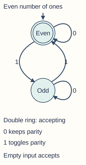
A deterministic complete recogniser for binary strings with an even number of ones. Even is both initial and accepting; 0 loops in each state and 1 switches states in either direction. Final acceptance is tested only after the whole input. The entry arrow consumes no symbol.
Parity state update — Original executed VB.NET fragment inside a module with Option Strict On and System/System.Text imports. This is the stated finite teaching example; its tests do not decide general language equivalence or program halting.
```
Public Function EvenOnes(input As String) As Boolean
    Dim even As Boolean = True
    For Each symbol As Char In input
        Select Case symbol
            Case "0"c ' Same state.
            Case "1"c : even = Not even
            Case Else : Throw New ArgumentException("Binary alphabet only")
        End Select
    Next
    Return even
End Function
```
Suffix recogniser — To recognise binary strings ending in 01, let q0 mean no useful suffix, q1 mean the latest symbol is 0 and accepting q2 mean the latest two end in 01. On 0, all states go to q1; on 1, q0→q0, q1→q2 and q2→q0. Thus 1101 accepts but 010 ends in q1 and rejects, even though it passed through q2 earlier.
Three-state suffix recogniser — Original executed VB.NET fragment inside a module with Option Strict On and System/System.Text imports. This is the stated finite teaching example; its tests do not decide general language equivalence or program halting.
```
Public Function Ends01Machine(input As String) As Boolean
    Dim state As Integer = 0
    For Each symbol As Char In input
        If symbol = "0"c Then
            state = 1
        ElseIf symbol = "1"c Then
            state = If(state = 1, 2, 0)
        Else
            Throw New ArgumentException("Binary alphabet only")
        End If
    Next
    Return state = 2
End Function
```
Constructing equivalent forms — To make a table from a diagram, check every state-symbol combination against its labelled edge. To design a machine, choose states representing just the past information needed for future decisions and test representative accepted/rejected strings, empty input and boundary patterns. State names are labels; changing names consistently does not change the recognised language.
Mealy outputs on transitions — A Mealy machine associates output with transitions, commonly labelled input/output. The produced value depends on the current state and incoming symbol, and the machine then changes state. Do not put an unexplained output solely inside a state and call it the same transition-output convention; trace emitted outputs as well as final state.
Mealy worked detector — A binary 01 detector can use No0 and Seen0. From No0, 0 gives Seen0/output 0 and 1 gives No0/output 0; from Seen0, 0 gives Seen0/output 0 and 1 gives No0/output 1. Starting No0, input 00101 emits 00101: output 1 marks each completed 01. This is an output sequence, not merely a final accept/reject answer.
Complete transition/output table for the two-state 01 detector. N=No0 and S=Seen0; an input 1 from S emits 1, all other transitions emit 0. The worked input 00101 emits 00101, identifying the two completed 01 pairs. These are transition outputs rather than values stored only inside states.
Transition-output detector — Original executed VB.NET fragment inside a module with Option Strict On and System/System.Text imports. This is the stated finite teaching example; its tests do not decide general language equivalence or program halting.
```
Public Function Detect01(input As String) As String
    Dim seenZero As Boolean = False
    Dim output As New StringBuilder()
    For Each symbol As Char In input
        If symbol <> "0"c AndAlso symbol <> "1"c Then Throw New ArgumentException("Binary alphabet only")
        output.Append(If(seenZero AndAlso symbol = "1"c, "1"c, "0"c))
        seenZero = (symbol = "0"c)
    Next
    Return output.ToString()
End Function
```

Regular expressions and regular languages

Regular-expression meaning — A theoretical regular expression describes a set of strings through literals, concatenation, alternation and repetition. In the printed notation here, the vertical-bar symbol ∣ means alternation. a(a∣b)* describes strings starting with a followed by any finite number of a or b symbols, including a alone. It does not mean start with any arbitrary character.
Concatenation and alternation — ab means a followed by b, whereas a∣b means either one-symbol string a or one-symbol string b. Grouping changes scope: (ab)∣c differs from a(b∣c). State the alphabet and grouping and use token boundaries carefully instead of interpreting the alternation sign as an instruction to include that character in the matched data.
Repetition operators — R* permits zero or more repetitions of R, R+ requires one or more and R? permits zero or one. Thus (ab)* allows ε,ab,abab,…, while (ab)+ excludes ε. These operators apply to the immediately preceding expression or group; ab* repeats b rather than the whole ab pair.
Worked pattern design — Over binary alphabet {0,1}, (0∣1)*01 recognises strings ending in 01. The repeated prefix can be empty, so 01 is accepted; 1101 is accepted and 010 is rejected. A suffix requirement is not equivalent to contains 01 somewhere: the rest of the pattern must account for the whole input.
Equivalent FSM and regex — Regular expressions and finite state recognisers define the same class of languages. The three-state suffix machine and (0∣1)*01 describe the same language. Test both on the same finite examples to find mistakes, while recognising that a few matching test outcomes alone do not prove equivalence for every possible string.
Regular-language limit — A finite number of states can record parity or a bounded suffix, but cannot retain an arbitrary exact unbounded count of earlier zeros to require the same number of later ones. The unbounded {0ⁿ1ⁿ : n ≥ 1} language is not regular. A finite maximum repetition bound changes the problem and can be represented by a sufficiently large finite machine.
Practical regex conventions — Programming regex libraries may add anchors, character classes, escaping or non-regular extensions beyond the course's theoretical operators. Check whether an API searches for a matching substring or requires the whole input. In .NET, an explicitly anchored full-string pattern using \A and \z can enforce start and absolute end; do not assume an unanchored IsMatch proves the entire string belongs to a language.

Context-free grammars, BNF and syntax diagrams

Productions and symbols — A grammar uses nonterminal categories, terminal symbols and production rules to describe valid strings from a start category. BNF means Backus–Naur form, a notation for writing grammar rules. In BNF, ::= means can be replaced by and alternatives can be separated by a vertical bar. Nonterminal names such as <digit> describe categories; their angle brackets are notation unless a grammar explicitly makes them literal input characters.
Simple numeric grammar — For a small alphabet, <digit> ::= 0 ∣ 1 ∣ 2 and <number> ::= <digit> ∣ <digit><number> generate one or more of the allowed digits. The string 120 is valid while 13 is not because 3 is outside this particular digit rule. Leading zeros are allowed by these productions unless an additional rule forbids them.
Derivation and checking — A derivation repeatedly replaces one nonterminal according to a production until only terminals remain. For 12, <number> ⇒ <digit><number> ⇒ 1<number> ⇒ 1<digit> ⇒ 12 is one derivation under the small numeric grammar. Check that every replacement is licensed; a string looking like an ordinary number does not override a restricted grammar's rules.
Recursion and balanced nesting — The grammar S ::= aSb ∣ ab generates ab,aabb,aaabbb,… with equal positive blocks of a then b. Each recursive expansion adds one a on the left and b on the right; the base production ends the process. This can express an unbounded matching-count relationship that a finite-state regular language cannot capture.
A grammar derivation S ⇒ aSb ⇒ aaSbb ⇒ aaabbb uses two recursive expansions and then the base production S ⇒ ab. It generates equal positive blocks of a then b, not arbitrary strings with equal symbol counts. S is a nonterminal, not a literal character in the completed string.
Recursive grammar checker for this language — Original executed VB.NET fragment inside a module with Option Strict On and System/System.Text imports. This is the stated finite teaching example; its tests do not decide general language equivalence or program halting.
```
Public Function MatchedBlocks(input As String) As Boolean
    ' Grammar S ::= aSb or ab, accepting positive blocks only.
    If input = "ab" Then Return True
    If input.Length < 4 OrElse input(0) <> "a"c OrElse input(input.Length - 1) <> "b"c Then Return False
    Return MatchedBlocks(input.Substring(1, input.Length - 2))
End Function
```
Syntax diagrams — A syntax diagram gives directed paths from entry to exit, with literal terminals and references to other syntax categories. Alternative branches express choice and loops express repetition under the diagram's rules. A legal string must follow a complete entry-to-exit route while satisfying referenced subdiagrams, not merely use some of the displayed symbols.
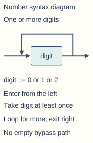
A syntax diagram for one or more occurrences of the nonterminal digit, whose rule permits 0,1,2. Entry from the left passes through digit at least once; the upper return path permits additional digits before exit right. The digit box refers to a subrule, not the literal five-letter input digit.
Syntax versus meaning — A grammar establishes allowed form, not every semantic property. A syntactically valid expression can still refer to an undeclared variable or divide by zero. Context-free grammar descriptions are more expressive than regular expressions for patterns such as unbounded nesting, but not every imaginable semantic requirement is solved just by writing BNF.

Functions, permutations and orders of growth

Functions as mappings — A mathematical function maps each member of a domain to exactly one output in a specified codomain. For f:ℕ→ℕ with f(n)=n+1, every supported natural input has one result. The image/range actually attained can be smaller than the codomain; a function is not required to use every allowed output or be implemented by one particular algorithm.
Linear and polynomial functions — A linear example is f(n)=2n+3; a quadratic example is g(n)=2n²+n. Both are polynomial, and their leading terms give usual growth classes O(n) and O(n²). A polynomial degree is fixed independently of n; nⁿ is not a fixed-degree polynomial merely because it contains the symbol n.
Exponential and logarithmic functions — For h(n)=2ⁿ, increasing n by one doubles the value. A logarithm reverses exponentiation: log₂8=3 because 2³=8. Changing a logarithm's fixed base multiplies it by a constant, so binary-search complexity is O(log n) without requiring every written logarithm to use exactly the same base.
Permutations and factorial — A permutation orders distinct objects. There are n! arrangements of n distinct items, where n!=n(n−1)…1 and 0!=1. Four distinct tasks have 24 possible orders; repeated identical objects change the counting model, so factorial of the printed length is not always the number of distinct word arrangements.
Deriving common loop costs — A fixed number of simple operations gives O(1). A loop over n items with constant work per item gives O(n); two independent nested n-pass loops give O(n²). A process repeatedly halving a positive problem size has logarithmically many stages. Dependent bounds need the actual count:1+2+…+n=n(n+1)/2 is still quadratic.
Compound and recursive work — Sequential costs add and the dominant growth governs the usual simplified bound; nested work often multiplies when the independent counts justify it. Merge sort's logarithmic levels each process linear total data, giving O(n log n). Do not label every recursion exponential or every pair of loops quadratic without examining the actual recurrence and bounds.
Space and practical limits — Compare working storage as well as steps, including retained arrays, queue entries and recursive frames. Better asymptotic growth can become decisive at scale, but hardware memory, constant factors, input encoding and desired precision still affect feasible runs. A faster processor improves a constant factor; it does not turn an exponential family into polynomial growth.

Tractability, heuristics and non-computability

Tractable and intractable problems — Under the course convention, a problem with a polynomial-or-better time solution is tractable; a problem with no polynomial-time solution is intractable. Distinguish a problem's best possible solution class from one inefficient algorithm chosen for it. A high-degree polynomial or enormous constant can still be impractical for a particular real input despite the classification.
Unknown versus proved limits — Failure to find a polynomial algorithm does not prove none exists. Some important complexity questions remain unresolved, so do not label every problem currently attacked by exhaustive search as mathematically proved intractable. State whether the claim concerns a supplied algorithm, a known upper bound or a proven problem limitation.
Heuristic methods — A heuristic uses a practical rule to obtain a useful answer without necessarily guaranteeing global optimality or the strongest exact property. Choosing a nearby unvisited stop can build a quick route but need not give the shortest complete tour. Evaluate speed, solution quality and failure cases against the objective instead of describing heuristic as random guessing or automatic proof.
Computable versus feasible — A computable problem has an algorithmic solution under the relevant formal model, even if the required time or storage makes large instances impractical. A non-computable/undecidable problem lacks a general deciding algorithm for all supported instances. Intractability and undecidability are different limits: very slow solvable problems are not thereby undecidable.
Halting problem — The general halting problem asks whether an arbitrary program with a specified input will eventually stop. No algorithm can always decide this correctly for every program-input pair. This does not prevent deciding many particular cases, such as an obvious finite counted loop, or useful analysis tools that sometimes return unknown.
Significance of undecidability — The halting limit is a theoretical restriction, not merely insufficient current memory, a slow processor or missing test data. Running a program for a long time without termination does not establish that it will never halt later. The course asks for a description and significance rather than a full formal proof; avoid claiming a timeout solves the general problem.

Turing machines and universal computation

Formal machine components — A Turing machine has a finite state control, finite symbol alphabet, tape divided into cells and a read/write head sensing one cell at a time. This course's examination model uses one tape infinite in one direction. A start state establishes initial control, and a halting state has no outgoing transition under the specified convention.
Transition function — A transition maps a current state and scanned symbol to a next state, symbol to write and head movement, such as δ(q,1)=(q,1,R). Here δ labels the transition function: in state q reading 1, remain in q, write 1 and move right (R) in this tuple convention. Use the exact supplied tuple order and movement notation. A finite rule table or transition diagram encodes the same machine; the unbounded tape is storage, not infinitely many control states.
Configuration and tracing — A configuration includes current state, relevant tape contents and head position. For each step read the scanned symbol, choose its rule, write the replacement, move one cell as directed and enter the next state. Record all changed parts rather than only the final tape, and respect the left boundary of a one-way-infinite tape instead of inventing negative cells.

Unary increment machine — Represent n by n consecutive 1 symbols starting at the leftmost cell, followed by blanks. In state Scan, reading 1 writes 1, moves R and stays Scan; reading blank writes 1, moves R and enters Halt. The result has n+1 ones. This machine never moves left, so it respects the one-way tape boundary even for n=0.

Finite simulation of this unary machine — Original executed VB.NET fragment inside a module with Option Strict On and System/System.Text imports. This is the stated finite teaching example; its tests do not decide general language equivalence or program halting.

Public Function IncrementUnary(input As String) As String
    ' Finite visible tape region for this fixed scan-right machine.
    ' '_' denotes blank. An extra blank permits the final right move.
    For Each symbol As Char In input
        If symbol <> "1"c Then Throw New ArgumentException("Unary ones only")
    Next
    Dim tape As New StringBuilder(input & "__")
    Dim head As Integer = 0
    Dim halted As Boolean = False
    While Not halted
        If tape(head) = "1"c Then
            head += 1
        ElseIf tape(head) = "_"c Then
            tape(head) = "1"c
            head += 1
            halted = True
        Else
            Throw New InvalidOperationException("No transition")
        End If
    End While
    Return tape.ToString().TrimEnd("_"c)
End Function

Worked tape trace — For initial tape 11□□… with head at cell 0 in Scan, the first rule leaves the tape unchanged and moves to cell 1. The second moves to cell 2; the blank rule writes 1 there and moves to cell 3 in Halt. The output 111 represents 3 in unary, not the binary number seven, because the input/output representation is part of the contract.
Initial and final configurations of the stated unary-increment Turing machine. Initially cells 0,1 contain 1 and head 0 is in Scan. After scanning and writing at the first blank, cells 0,1,2 contain 1, head 3 is in Halt. Only a finite tape window is drawn; blanks continue to the right and the model has no negative-index cells.
Computability model — Turing machines provide a precise general model for what an effective algorithm can compute. Their purpose is not to be a fast physical design or a claim that an actual machine owns infinite memory. Finite real machines can simulate bounded portions, while the idealised unbounded model separates logical computability from practical resource limits.
Universal Turing machine — A universal Turing machine interprets an encoded description of another machine together with its input and simulates that machine's computation. This separates the simulator's fixed program from the represented program data. Universality does not make halting decidable or promise that every simulated computation will finish.

K5CS4 · Abstraction, languages and computation