K5CS3 · Algorithms, search, traversal and optimisation · AQA A-level Computer Science (VB.NET)

Revise the key ideas

Algorithm contracts, tracing and complexity

Algorithm and contract — An algorithm gives sufficiently precise steps for solving a defined class of problems. State the inputs, promised result and necessary preconditions, conditions that must already hold before the algorithm starts: binary search needs data ordered under the same comparison used by the search. A trace that happens to find one item in unsorted data does not remove that requirement.
Tracing state and output — Record relevant variables, collection contents, visited/settled state and produced output after each specified operation. Distinguish an item discovered from one processed, and a returned value from data remaining in the structure. Use the supplied algorithm's exact update order rather than replacing it with a remembered variant that may produce a different valid traversal order.
Correctness and invariants — A loop invariant is a property maintained at a defined point in each iteration, such as a possible search interval containing every remaining candidate. Explain initial truth, preservation by an iteration and how termination yields the required result. Testing provides examples of behaviour; an invariant argument can explain why the method works for a whole input class under its assumptions.
Input size and operation counts — Choose a meaningful input-size measure such as number of elements n or graph vertices V and edges E. Count the relevant comparisons, updates or traversed entries under a declared model. A fixed clock timing also depends on hardware, implementation and data, so one measured run is not an abstract time-complexity proof.
Growth and Big O — Big O describes an asymptotic upper bound on growth, describing a limit on how the work grows as input size becomes large, under a specified case and cost model. Typical comparisons use constant O(1), logarithmic O(log n), linear O(n), linearithmic O(n log n) and quadratic O(n²). Doubling n roughly doubles a linear leading term but roughly quadruples a quadratic one; constants and lower-order work can still matter for small actual inputs.
Best, worst and space cases — State which input case a bound concerns and distinguish time from auxiliary space, extra working memory beyond the input itself. Linear search can succeed on its first comparison but has linear worst-case work. A loose upper bound is not necessarily a tight description; when teaching the usual named classes, explain the actual dominant work instead of assuming every O notation means exact equality or always worst case.

Breadth-first graph traversal

Breadth-first idea — Breadth-first search explores a start vertex, then its undiscovered neighbours, then successive layers of neighbours. An ordinary FIFO queue preserves this layer progression. In a graph containing cycles, an explicit discovered/visited set prevents endless revisiting and repeated insertion of the same vertex.

BFS procedure — Mark the start discovered and enqueue it. While the queue is nonempty, dequeue a vertex, process it and examine its outgoing neighbours in the specified order; mark and enqueue each still-undiscovered neighbour. Marking on enqueue prevents two already queued parents from independently adding the same neighbour before either processes it.

BFS with discovery on enqueue — Original executed VB.NET fragment, inside a module with Option Strict On and System/System.Collections.Generic imports. Use its stated preconditions and supported grammar.

Public Function BreadthFirst(graph As Dictionary(Of String, String()), start As String) As List(Of String)
    Dim output As New List(Of String)()
    Dim discovered As New HashSet(Of String)()
    Dim waiting As New Queue(Of String)()
    discovered.Add(start) : waiting.Enqueue(start)
    While waiting.Count > 0
        Dim current As String = waiting.Dequeue()
        output.Add(current)
        For Each neighbour As String In graph(current)
            If discovered.Add(neighbour) Then waiting.Enqueue(neighbour)
        Next
    End While
    Return output
End Function

BFS worked trace — Use undirected edges A–B, A–C, B–D, C–D and C–E, with neighbours considered alphabetically and start A. After processing A, queue [B,C]; after B, [C,D]; after C, [D,E], because D is already discovered. Processing D then E empties the queue. The processing order is A,B,C,D,E.
The worked undirected cyclic graph has edges A-B,A-C,B-D,C-D,C-E. With start A and alphabetical neighbours, FIFO BFS processes A,B,C,D,E, whereas recursive DFS visits A,B,D,C,E. The cycle makes the visited/discovery convention essential; the diagram fixes neighbour order, not a universal traversal order.
BFS distances and predecessors — Set the start distance to 0; when discovering a neighbour from u, assign distance(u)+1 and predecessor u. In the worked graph, B,C have distance 1 and D,E distance 2. Following predecessors from a target back to the start reconstructs a shortest path in edge count; reverse that collected route for forward presentation.
Shortest unweighted paths — BFS's layer invariant ensures the first discovery distance is minimum edge count for vertices reachable from the chosen start in an unweighted graph, or minimum total cost if every edge has the same positive cost. It does not minimise arbitrary different weights. Direction matters: follow allowed outgoing edges rather than inventing reverse travel.
Disconnected graphs and uses — A BFS from one start visits only its reachable component/region. To traverse every vertex of a disconnected graph, restart from each undiscovered vertex under a declared outer order. Applications include finding a fewest-hop route and exploring degrees of connection; a reachable target is not guaranteed merely because it appears somewhere in the input graph.
BFS resources — With adjacency lists and each vertex marked once, traversal work is O(V + E) across the visited graph and storage for queue/marks is O(V). A matrix scan can inspect V potential neighbours for every processed vertex, producing O(V²) work. The choice of representation changes the cost, not the core FIFO exploration rule.

Depth-first graph traversal

Depth-first idea — Depth-first search follows one not-yet-visited route as far as possible before backtracking to an earlier branching point. It can use recursion or an explicit LIFO stack, with a visited set for graphs with cycles. Backtracking means resuming unexplored alternatives, not forgetting that already visited vertices exist.
Recursive DFS procedure — On entering Visit(v), mark v, process it, then call Visit on each still-unvisited outgoing neighbour in the specified order. A recursive call returns when that branch has no remaining undiscovered neighbour, resuming the caller's loop. Separate call frames retain the pending branch work.
Recursive DFS with ordered input neighbours — Original executed VB.NET fragment, inside a module with Option Strict On and System/System.Collections.Generic imports. Use its stated preconditions and supported grammar.
```
Public Sub DepthVisit(graph As Dictionary(Of String, String()), current As String, visited As HashSet(Of String), output As List(Of String))
    visited.Add(current) : output.Add(current)
    For Each neighbour As String In graph(current)
        If Not visited.Contains(neighbour) Then DepthVisit(graph, neighbour, visited, output)
    Next
End Sub
```
DFS worked trace — For the same undirected graph A–B, A–C, B–D, C–D, C–E with alphabetical neighbours, recursive DFS from A visits A,B,D,C,E. At D, B is already visited, so C is the next unvisited neighbour. At C, both A and D are visited; E is explored before returning through the pending calls.
Iterative stack variants — An explicit-stack DFS can push unvisited neighbours and process the most recently pushed next. Pushing alphabetical neighbours in ascending order can lead to a different order from recursive ascending-neighbour DFS; reverse push order can help match it, depending on the marking/stack-frame convention. Trace the given algorithm and state tie/neighbour rules rather than asserting one universal DFS order.
Applications and limits — DFS can explore a maze and support backtracking, reachability and structural analysis. It does not generally find a path with the fewest edges or lowest weight on first discovery. Finding a valid route is a different promise from finding an optimal route, and returning to a branching point may be necessary when a branch fails.
Cycle handling and resources — Mark a vertex before exploring its neighbours so a cycle such as A–B–D–C–A does not recur forever. Standard adjacency-list DFS uses O(V + E) work and O(V) visited/call-or-explicit-stack storage in the worst case. A very deep graph can exhaust a language call stack even though the graph is finite.

Binary-tree traversal and applications

Traversal versus search — A tree traversal systematically visits relevant nodes; a comparison-based search may follow only one branch toward a key. Empty child references are base cases in recursive traversal. Specify whether a node's processing happens before, between or after its child traversals, since that choice defines the output order.
Pre-order — Pre-order visits node, then left subtree, then right subtree. For root 8, children 3 and 10, and children 1 and 6 under 3, the order is 8,3,1,6,10. Visiting a parent before children can support copying a rooted structure when the parent context must be established first.
In-order — In-order visits left subtree, then node, then right subtree in a binary tree. For the same example the order is 1,3,6,8,10. This is ascending key order because the example satisfies a binary search-tree invariant; an arbitrary binary tree's in-order sequence is not necessarily sorted.
Post-order — Post-order visits left subtree, then right subtree, then node. The example gives 1,6,3,10,8. It supports tasks in which child results or cleanup must precede their parent, including evaluating an expression tree or generating its postfix form. The recursive structure and absent-child checks matter more than memorising one sequence.
Expression trees — For (3 + 4) × 2, use multiplication at the root, a plus node as its left child with leaves 3 and 4, and leaf 2 as its right child. Pre-order gives prefix * + 3 4 2; post-order gives postfix 3 4 + 2 *. In-order needs appropriate parentheses to preserve the original grouping rather than printing ambiguous 3 + 4 * 2.
Expression tree for (3+4)*2: plus combines 3 and 4 before the root multiplication combines that result with 2. Post-order emits 3 4 + 2 *. A bare in-order token stream without grouping brackets could instead mean 3+(4*2), so reconstruct infix with appropriate parentheses.
Traversal work and representation — A full traversal visits each of n nodes once, so ordinary traversal work is O(n) when processing per node is constant. Recursive auxiliary call depth is the tree height, which can be O(log n) for a suitably balanced tree but O(n) for a chain. Copying or emitting output itself requires storage appropriate to the produced result.

Reverse Polish notation and expression stacks

Infix and postfix — In infix notation an operator lies between operands; in Reverse Polish/postfix notation the operator follows its operands. A + B becomes A B + and (A + B) * C becomes A B + C *. With known operator arity, the number of operands an operator requires, and correctly separated tokens, postfix gives evaluation order without grouping brackets.
Precedence and grouping — A + B * C becomes A B C * +, because multiplication combines B and C before addition. (A + B) * C becomes A B + C * instead. Token order preserves the expression tree's meaning; dropping parentheses from an infix string is not a conversion algorithm.
Operator-stack conversion — A standard infix-to-postfix method emits operands immediately and keeps pending operators on a stack. On a new operator, pop operators of higher precedence, and equal precedence when the new operator is left-associative; then push the new operator. A left bracket is pushed, while a right bracket triggers popping until the matching left bracket, which is removed without output.
Associativity and token rules — For left-associative subtraction, A − B − C means (A − B) − C and gives A B − C −. Right-associative exponentiation needs a different equal-precedence rule. Tokenise multi-digit numbers and names; unary minus or function calls need explicit additional rules and cannot safely be guessed from an algorithm stated only for binary operators.

Postfix evaluation — Read tokens left to right. Push an operand value; for a binary operator pop the right operand first, then the left, calculate left operator right and push the result. For 10 3 − the result is 7, not −7. An operator needing two items when fewer are available indicates an invalid expression under this grammar.

Postfix numeric evaluator — Original executed VB.NET fragment, inside a module with Option Strict On and System/System.Collections.Generic imports. Use its stated preconditions and supported grammar.

Public Function EvaluatePostfix(tokens() As String) As Double
    ' Grammar: invariant-culture numeric tokens and binary +,-,*,/ only.
    Dim values As New Stack(Of Double)()
    For Each token As String In tokens
        Dim number As Double
        If Double.TryParse(token, Globalization.NumberStyles.Float, Globalization.CultureInfo.InvariantCulture, number) Then
            values.Push(number)
        Else
            If values.Count < 2 Then Throw New FormatException("Too few operands")
            Dim right As Double = values.Pop(), left As Double = values.Pop()
            Select Case token
                Case "+" : values.Push(left + right)
                Case "-" : values.Push(left - right)
                Case "*" : values.Push(left * right)
                Case "/"
                    If right = 0 Then Throw New DivideByZeroException()
                    values.Push(left / right)
                Case Else : Throw New FormatException("Unsupported token")
            End Select
        End If
    Next
    If values.Count <> 1 Then Throw New FormatException("Expected one result")
    Return values.Pop()
End Function

Worked evaluation — For 3 4 + 2 *, the operand stack evolves [3], [3,4], [7], [7,2], [14], with the top at the right. Addition replaces its two operands with 7 before multiplication uses 7 and 2. A valid completed expression under the stated binary grammar leaves exactly one result, not leftover unused operands.
After each token in 3 4 + 2 *, the stack is [3],[3,4],[7],[7,2],[14], with its top on the right. A binary operation replaces two operands with one result. Operand order is especially important for subtraction/division; a complete valid expression leaves one result.
Postfix to infix — A stack of expression strings can reconstruct infix: push operands and, on an operator, pop right then left and push a parenthesised (left operator right). For A B C * + this produces (A + (B * C)). Parentheses can later be reduced only when precedence/associativity preserves the same meaning.
Why postfix is useful — Postfix suits stack-based evaluation in interpreters and virtual-machine instruction models. It avoids needing to resolve infix precedence during that evaluation step, because conversion has already encoded the grouping. It is still a representation requiring valid syntax and operand types; no bracket characters does not mean malformed expressions cannot exist.

Linear and binary search

Linear search — Linear search compares successive elements with a target until a match or the end. It can work with unsorted data and, under a first-match contract, returns the first matching index. For [7,2,9,2] searching 2 gives index 1 in zero-based notation; finding every match requires continuing rather than returning immediately.
First-match linear search — Original executed VB.NET fragment, inside a module with Option Strict On and System/System.Collections.Generic imports. Use its stated preconditions and supported grammar.
```
Public Function LinearSearch(items() As Integer, target As Integer) As Integer
    For i As Integer = 0 To items.Length - 1
        If items(i) = target Then Return i
    Next
    Return -1
End Function
```
Linear-search limits — An unsuccessful search may compare all n elements, giving O(n) worst-case work; a first-element success uses constant work. No-match can return a documented sentinel such as −1, which must not be used as an ordinary index. Include empty data, last-element and missing-target cases when testing.
Binary-search precondition — Binary search repeatedly narrows an ordered candidate interval by comparing its middle item. The ordering and comparison must be consistent, and efficient direct middle access is assumed for the usual array model. Sorting once may benefit many later searches, but sorting an entire changing dataset for one tiny lookup may cost more overall than a linear scan.
Inclusive-bound algorithm — Start low = 0 and high = length − 1. While low ≤ high, set mid = low + (high − low) \ 2 for nonnegative integer interval length; compare items(mid) with target. On smaller middle value move low to mid + 1; on larger move high to mid − 1; on equality return mid. If the interval empties, return the documented no-match result.
Inclusive-bound binary search — Original executed VB.NET fragment, inside a module with Option Strict On and System/System.Collections.Generic imports. Use its stated preconditions and supported grammar.
```
Public Function BinarySearch(items() As Integer, target As Integer) As Integer
    ' Precondition: ascending sorted array using this numeric comparison.
    Dim low As Integer = 0, high As Integer = items.Length - 1
    While low <= high
        Dim mid As Integer = low + (high - low) \ 2
        If items(mid) = target Then Return mid
        If items(mid) < target Then
            low = mid + 1
        Else
            high = mid - 1
        End If
    End While
    Return -1
End Function
```
Worked binary trace — For sorted [2,5,8,12,16,23,38] searching 16, low=0 and high=6 give mid 3, value 12. Move low to 4; now mid 5, value 23, so high becomes 4. Then mid 4 holds 16 and the search succeeds at index 4. Record actual indices and values separately so midpoint arithmetic is auditable.
Inclusive-bound binary search for 16 in the stated seven-element ascending array examines indices 3,5,4 and values 12,23,16. The interval changes 0..6 to 4..6 to 4..4. A failed comparison excludes the middle with mid+1 or mid-1, ensuring the search progresses.
Why the interval shrinks — After a comparison, sorted order rules out the middle element and the entire unsuitable side. Using mid + 1 or mid − 1 excludes the already tested middle and guarantees progress for a nonempty interval. Updates that leave low = mid in a two-element case can repeat the same midpoint and fail to terminate.
Binary-search costs and duplicates — Each comparison roughly halves the remaining interval, giving O(log n) worst-case array search and O(1) auxiliary space for an iterative version. A recursive version uses call-stack space. With duplicate keys an ordinary match-return algorithm may return any matching index; finding the first or last occurrence requires a modified contract and continued boundary search.

Binary search-tree search

Following the ordering invariant — Begin at the root. Compare the target key with the node: on equality succeed, on smaller follow the left child, on larger follow the right child. Reaching an absent child means no match under the tree invariant. This search is valid for a correctly ordered binary search tree, not any binary-shaped hierarchy.
Worked tree search — In the tree rooted 8, with left child 3, right child 10 and 3's children 1 and 6, searching 6 compares 8, then 3, then 6. Searching 7 follows 8→3→6 then the absent right child and fails. The search does not also scan 10 or 1 because the subtree ordering excludes them.
Height determines cost — Search work is proportional to the followed path height. The familiar O(log n) analysis assumes a suitably balanced tree; an unbalanced chain can require O(n) worst-case comparisons. AQA's headline logarithmic tree-search classification should be understood with that shape assumption, not taught as an unconditional guarantee for every binary search tree.
Duplicates and maintenance — Choose and maintain a duplicate-key rule, such as reject repeated keys or store a count in a matching node. Insertion, deletion and any rebalancing must preserve the ordering and reference structure before later search is trusted. A successful example lookup does not prove all paths or every node satisfy the invariant.

Bubble sort

Adjacent comparison method — For ascending bubble sort, scan adjacent pairs and swap an out-of-order pair. After a complete left-to-right pass, a largest remaining item reaches the right boundary of the active region. The algorithm repeatedly shrinks that region until all required passes finish or an explicitly implemented no-swap condition establishes completion.
Worked first pass — Starting [5,1,4,2], compare 5/1→[1,5,4,2], compare 5/4→[1,4,5,2], then 5/2→[1,4,2,5]. The final 5 is in its sorted position, but the entire array is not yet sorted because 4 precedes 2. State the pass direction; a different valid variant may move small values toward the left instead.
Remaining passes and invariant — The next active pass compares 1/4 without swap and 4/2 with swap, giving [1,2,4,5]. A final required check or the implemented pass logic establishes completion. The right-hand suffix is already sorted after each pass, so repeated comparisons inside that suffix can be excluded under the shrinking-bound implementation.
Optimised stopping and complexity — A swapped flag reset at each pass allows early stopping after a pass with no swaps. This optimised version has O(n) best-case work on already sorted data, while average/worst work remains O(n²). A fixed-pass version can remain quadratic even on sorted input. State the implementation rather than treating the best case as the same for every variant.
Bubble sort with no-swap stopping — Original executed VB.NET fragment, inside a module with Option Strict On and System/System.Collections.Generic imports. Use its stated preconditions and supported grammar.
```
Public Sub BubbleSort(items() As Integer)
    For boundary As Integer = items.Length - 1 To 1 Step -1
        Dim swapped As Boolean = False
        For i As Integer = 0 To boundary - 1
            If items(i) > items(i + 1) Then
                Dim temporary As Integer = items(i)
                items(i) = items(i + 1)
                items(i + 1) = temporary
                swapped = True
            End If
        Next
        If Not swapped Then Exit For
    Next
End Sub
```
Space and stability — In-place means rearranging items in the original storage rather than building a complete separate output. In-place adjacent swapping uses constant auxiliary storage for the usual array implementation. Swapping only when left > right preserves the original order of equal keys, making this version stable. Swapping equals unnecessarily can destroy stability; sorting candidate records by score may need equal-score arrival order preserved.
Testing bubble sort — Check empty, single-item, already sorted, reverse-sorted, duplicate and negative-key inputs, preserving any record payload attached to keys. Independently verify both nondecreasing output and preservation of the input multiset, all the original values together with how many times each occurs; an array full of one repeated minimum is ordered but is not a correct sort of arbitrary original data.

Merge sort and divide and conquer

Divide and conquer — Merge sort divides a sequence into smaller parts, sorts them recursively and combines their sorted results through merging. A sequence of length 0 or 1 is already sorted under the usual base case. Division alone does not produce sorted output: the merge stage must preserve every element and the ordering invariant.

Merging two sorted runs — Use one index for each sorted run. Repeatedly take the smaller current item into the output, advance only that run's index, then append all remaining items once one run is exhausted. Both inputs must already be sorted under the same comparison. Repeatedly restarting a full scan is not the ordinary linear merge.

Merge-sort and two-run merge fragments — Original executed VB.NET fragment, inside a module with Option Strict On and System/System.Collections.Generic imports. Use its stated preconditions and supported grammar.

Public Function MergeSort(items() As Integer) As Integer()
    If items.Length <= 1 Then Return DirectCast(items.Clone(), Integer())
    Dim split As Integer = items.Length \ 2
    Dim left(split - 1) As Integer
    Dim right(items.Length - split - 1) As Integer
    Array.Copy(items, 0, left, 0, left.Length)
    Array.Copy(items, split, right, 0, right.Length)
    Return Merge(MergeSort(left), MergeSort(right))
End Function
Public Function Merge(left() As Integer, right() As Integer) As Integer()
    Dim output(left.Length + right.Length - 1) As Integer
    Dim i As Integer = 0, j As Integer = 0, k As Integer = 0
    While i < left.Length AndAlso j < right.Length
        If left(i) <= right(j) Then
            output(k) = left(i) : i += 1
        Else
            output(k) = right(j) : j += 1
        End If
        k += 1
    End While
    While i < left.Length
        output(k) = left(i) : i += 1 : k += 1
    End While
    While j < right.Length
        output(k) = right(j) : j += 1 : k += 1
    End While
    Return output
End Function

Worked split and merge — For [5,1,4,2], split into [5,1] and [4,2], then singletons [5],[1],[4],[2]. Merge to [1,5] and [2,4], then compare 1/2,5/2,5/4 and append remaining 5 to obtain [1,2,4,5]. A trace should show both the split hierarchy and the actual comparisons during combination.
Split/merge hierarchy for [5,1,4,2]. Two pairs divide into singletons, then merge into [1,5] and [2,4], and finally [1,2,4,5]. Arrows in the upper half show decomposition and lower arrows show combination; no item is lost or duplicated.
Time-complexity reasoning — A balanced split tree has about log₂n levels, and the total elements merged across one level are n, giving O(n log n) usual merge-sort work. Merging one pair of runs with lengths a and b is O(a + b). Multiplying every level's cost by an extra n would double-count work and incorrectly produce quadratic analysis.
Storage and stability — A conventional array merge sort uses O(n) auxiliary merge storage plus logarithmic recursive depth. It is not automatically an O(1)-space in-place method. Choosing the left run first for equal keys preserves original equal-key order, yielding a stable implementation; the exact space and stability claims depend on the actual variant.
Comparing sorting choices — Merge sort's growth can suit larger datasets, while an optimised bubble sort is simple and may stop quickly on already ordered short input. Actual constants, memory constraints, input pattern and required stability matter. Big O helps compare scaling but does not guarantee one concrete implementation wins every timing at every small n.

Dijkstra shortest paths and optimisation

Problem and preconditions — Dijkstra's method finds minimum-total-weight routes from a chosen start under the standard nonnegative-edge-weight assumption. Directed edges must be followed in their permitted direction. Negative edges invalidate the usual settled-distance guarantee, while zero-weight edges can be allowed; fewest edges is a different objective from minimum weight.
Tentative distance setup — Give the start tentative distance 0, every other vertex infinity/unknown and no predecessor. Maintain which vertices are not yet settled. A tentative distance is the best route cost discovered so far, not necessarily final merely because it has a finite value or has been written first.
Choose and relax — Select an unsettled reachable vertex u of smallest tentative distance and settle it. For each relevant outgoing edge u→v of weight w to an unsettled neighbour, compare distance(u)+w with v's current value; if smaller, replace the tentative distance and predecessor. Relaxation means testing a better route, not simply adding the new weight to every old tentative value.
Worked graph and first steps — Use an undirected graph with edges A–B: 4, A–C: 1, C–B: 2, C–D: 5, B–D: 1, D–E: 3, B–E: 7 and C–E: 10. Settle A at 0, giving B = 4, C = 1. Settle C at 1, improving B to 3, D to 6 and E to 11. These figures are calculated illustrative weights, not measured travel times.
Worked completion — Next settle B at 3: D improves to 4 through B and E to 10 through B. Settle D at 4: E improves to 7. Finally settle E at 7. Final costs from A are A = 0, C = 1, B = 3, D = 4, E = 7, and the shortest route to E follows A→C→B→D→E with total 1+2+1+3=7.
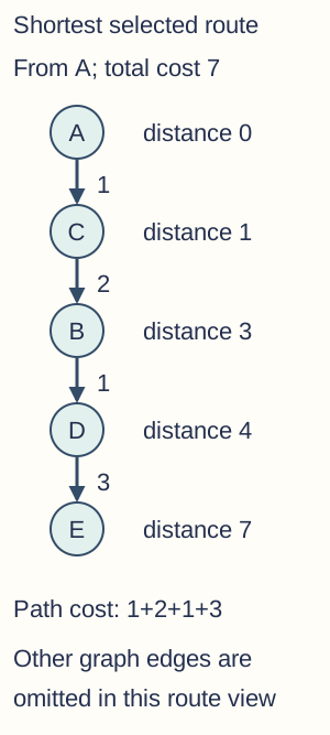
The chosen shortest route in the full worked weighted graph is A-C-B-D-E, with edge costs 1,2,1,3 and cumulative distances 0,1,3,4,7. This route view deliberately omits other graph edges and is not the complete graph on which Dijkstra was run. Predecessors run backwards from E to A.
Predecessors and route reconstruction — Record a predecessor when a genuinely shorter tentative route replaces an old one. For E, follow E←D←B←C←A and reverse the sequence for forward travel. A distance table alone gives the cost, not automatically the complete route; equal-cost alternatives may produce different valid predecessor trees depending on tie policy.
Why settlement is safe — With nonnegative weights, a later route through a not-yet-settled vertex cannot improve the smallest tentative distance already selected for settlement. This is the key reason a settled value is final in the standard algorithm. Merely drawing a vertex in a permanent column is not a proof when the weight assumptions or minimum-selection rule are broken.
Unreachable vertices and stopping — If the smallest remaining tentative distance is infinity, the remaining vertices are unreachable from the start and no finite route should be invented. A run concerned only with one target may stop when that target is settled, not merely when first discovered. Continue further when all-start distances are required by the question.
Applications, costs and assessment — Weighted route planning, communication costs and network optimisation can use shortest-path models when their assumptions fit. A simple matrix/linear-selection implementation can take O(V²), while an appropriate adjacency-list/priority-queue version has different bounds and overhead. AQA requires understanding and tracing Dijkstra; its specification says the steps need not be recalled from memory, so practise the supplied method accurately rather than inventing a recall requirement.

K5CS3 · Algorithms, search, traversal and optimisation