K5CS2 · Data structures, files and vectors · AQA A-level Computer Science (VB.NET)

Revise the key ideas

Data structures, abstract types and storage choices

Structure and operations — A data structure organises related data so a program can perform operations such as access, insertion, deletion, search and traversal. Choose a representation from the required operations and constraints: a collection of scores, a queue of print jobs and a road graph need different relationships. A structure is not useful merely because its name sounds more advanced.
Abstract data type — An abstract data type describes the permitted values and operations through their behaviour, independently of one implementation. A stack promises last-in-first-out push/pop/peek behaviour; it may be implemented with an array or linked nodes. ADT abbreviates abstract data type. The same representation can support different ADTs, and the same ADT can have different time and memory trade-offs.
Static and dynamic structures — A static structure has a size or storage organisation fixed for the relevant allocation, while a dynamic structure can grow or shrink as the program runs. A fixed array gives predictable indexed storage but can reserve unused capacity or become full. Linked allocation can adapt to changing item counts but adds reference/storage overhead and may lose direct index access.
Capacity versus logical size — Capacity is the number of elements storage can hold; logical size is the number currently in use. An array-backed collection can have capacity 20 with only 6 live items. Maintain size and bounds explicitly so a traversal does not treat unused default values as real records; zero can be a legitimate value rather than an empty marker.
Resizing and allocation — An array-backed dynamic list may allocate a larger array and copy items when capacity is exhausted. An individual resize can be expensive even when average append cost over many operations is low. Dynamic does not mean every operation is constant time or that memory is unlimited; explain the actual implementation and workload.
Linked representations — A linked node can store data and references to other nodes, with an entry reference identifying the start. Insertion can relink nodes without shifting every later array element when the relevant position is already known. Finding that position can still need traversal; keeping references consumes storage, and a broken link can lose access to remaining nodes.
Choosing a model — Specify ordering, duplicates, key uniqueness, access frequency, maximum size and required operations before selecting a structure. A dictionary suits lookup by candidate code, a queue suits arrival order and a graph suits many-to-many connections. Justify time, memory and ease of correct implementation against the problem rather than treating one data structure as universally best.

One-dimensional and multidimensional arrays

Indexed arrays — An array selects elements through integer indices under a declared bound convention. Dim values(4) As Integer creates five VB.NET elements indexed 0 to 4. Traverse the actual logical range, and distinguish the array's length from its last index so an extra values(values.Length) access is not attempted.
Two-dimensional arrays — Dim board(2,3) As Integer creates a rectangular 3 by 4 array in VB.NET: row indices 0–2 and column indices 0–3. board(1,2) identifies one element using an ordered pair of indices. A row/column swap can compile and still refer to the wrong cell; document what each dimension represents.
Nested traversal — Use an outer loop over the first dimension and an inner loop over the second, with GetLength(0) and GetLength(1) or the appropriate upper bounds. A 3 by 4 rectangular array has 12 elements. For a row total, reset the row accumulator at the start of each row rather than accidentally carrying the preceding row's sum forward.
Dimensions and tuples — An n-dimensional array uses an ordered tuple of n indices, a group of n values kept in a defined order. A 3-dimensional model might identify room, day and period; changing their order changes the selected element. The number of stored elements is the product of dimension lengths for a rectangular array, subject to actual bounds and storage limits.
Rectangular versus jagged — A rectangular two-dimensional array has one consistent length for each dimension; an array of arrays can have separately allocated rows with different lengths. A jagged representation is not automatically interchangeable with a rectangular matrix. Traverse each existing inner array's own valid bounds and handle missing rows if the model permits them.
Parallel arrays versus records — Parallel arrays can store codes and scores at matching indices, but every insertion, deletion and sort must preserve their alignment. A record or class can group one candidate's fields and an array can hold those entities. Choose the model that makes the relationship explicit and reduces accidental mismatches.

Fields, records, text files and binary files

Fields and records — A field holds one named attribute, such as candidate code or score; a record groups the fields describing one entity. A file persists encoded data beyond the lifetime of an in-memory array. Decide a file format and field rules so the reader can reconstruct the intended records rather than treating arbitrary bytes as self-describing objects.
Text file representation — A text file encodes characters using a specified scheme such as UTF-8. A delimiter is a separator such as a comma or tab marking field boundaries. Lines and delimiters are format conventions rather than automatic guarantees of valid records. Specify how to handle headers, blank lines, quoting and embedded separators; blindly splitting every comma cannot correctly read all quoted CSV data.

Reading text safely — A StreamReader can read one line at a time until ReadLine returns Nothing, while an empty string can be a valid empty line. Using…End Using disposes the stream on normal control leaving the block, including relevant exceptions. Check file access failures meaningfully and do not confuse end-of-file with an invalid numeric field.

Read and validate simple text records — Original VB.NET with Option Strict On, inside the example module. File fragments need System.IO, System.Text and System.Collections.Generic imports as used in the retained source. Work only with deliberate practice files.

Public Function ReadTextScores(path As String) As List(Of Integer)
    Dim result As New List(Of Integer)()
    Using reader As New StreamReader(path, Encoding.UTF8)
        Dim line As String = reader.ReadLine()
        While line IsNot Nothing
            If line.Length > 0 Then
                Dim fields() As String = line.Split(ChrW(9))
                Dim score As Integer
                If fields.Length <> 2 OrElse fields(0).Length = 0 Then
                    Throw New FormatException("Expected code and score")
                End If
                If Not Integer.TryParse(fields(1), score) OrElse score < 0 OrElse score > 100 Then
                    Throw New FormatException("Invalid score")
                End If
                result.Add(score)
            End If
            line = reader.ReadLine()
        End While
    End Using
    Return result
End Function

Writing and appending text — A StreamWriter can write text lines to a chosen path. A normal overwrite-mode write replaces the file's previous contents, whereas an explicit append mode adds after existing content. Choose deliberately, encode consistently and close/dispose the writer so buffered output is flushed, meaning data held temporarily in memory is passed on to the underlying output stream; opening a file is not proof all intended output has been persisted.
Choose overwrite or append explicitly — Original VB.NET with Option Strict On, inside the example module. File fragments need System.IO, System.Text and System.Collections.Generic imports as used in the retained source. Work only with deliberate practice files.
```
Public Sub WriteTextScores(path As String, append As Boolean)
    Using writer As New StreamWriter(path, append, New UTF8Encoding(False))
        writer.WriteLine("00142" & vbTab & "73")
    End Using
End Sub
```
Parsing persisted records — For a deliberately simple two-field tab-separated teaching format with no tabs inside fields, split the line into exactly two fields, preserve the code as String and TryParse the score. Then check the allowed score range and duplicate-code policy. A valid character encoding does not prove the record satisfies the application's constraints.

Binary file representation — A binary file stores bytes interpreted according to an agreed format, often avoiding text conversion for numeric values. A BinaryWriter and matching BinaryReader can write and read declared types in the same order. Binary data is not encryption: someone who knows the format can interpret it, and a different field order/type can produce nonsense or failure.

Matching binary write/read fragments — Original VB.NET with Option Strict On, inside the example module. File fragments need System.IO, System.Text and System.Collections.Generic imports as used in the retained source. Work only with deliberate practice files.

Public Sub WriteBinaryScore(path As String)
    Using writer As New BinaryWriter(File.Open(path, FileMode.Create), Encoding.UTF8)
        writer.Write("00142") ' Length-prefixed string, not a fixed-width field.
        writer.Write(CInt(73))
    End Using
End Sub
Public Function ReadBinaryScore(path As String) As Integer
    Using reader As New BinaryReader(File.OpenRead(path), Encoding.UTF8)
        Dim code As String = reader.ReadString()
        Dim score As Integer = reader.ReadInt32()
        If code <> "00142" OrElse score < 0 OrElse score > 100 Then
            Throw New FormatException("Unexpected code or score")
        End If
        If reader.BaseStream.Position <> reader.BaseStream.Length Then
            Throw New FormatException("Unexpected trailing data")
        End If
        Return score
    End Using
End Function

Binary field sizes and framing — A chosen Int32 uses four bytes, but strings written by BinaryWriter are length-prefixed encoded sequences, with their encoded byte length written before the string data, and are not one universal fixed width. Record boundaries must follow the actual format. Do not multiply record number by a guessed fixed size when records contain variable-length strings; use an index or genuinely fixed-width encoding if random record access is required.
Sequential and random access — Sequential access processes records in file order, often suitable for a complete scan. Random access seeks to a known byte offset, a distance measured in bytes from a specified file position such as its start, useful when a format/index makes the target position calculable. For zero-based fixed records of 12 bytes after a 16-byte header, record index 5 begins at 16 + 5 × 12 = 76; this formula does not apply to arbitrary text lines.
Reliability and evidence — Validate counts, expected lengths and supported format versions before trusting a file, and handle incomplete or corrupted input. Tests should include empty files, malformed fields, missing paths and an overwrite/append distinction using disposable test fixtures. Do not demonstrate file handling by modifying real user data or claiming successful output without reading it back.

Linear, circular and priority queues

Queue abstraction — An ordinary queue removes the earliest still-waiting arrival first: first in, first out. Enqueue adds at the rear, dequeue removes at the front and a peek can inspect the front without removal. Print jobs or breadth-first search illustrate arrival-order processing; a priority queue uses an additional service rule and should not be described as universally ordinary FIFO.
Linear array queue — A linear queue can store elements in an array with front and rear positions. Under one declared convention, front identifies the next item, rear the next free slot and count the number of live items. Enqueue writes at rear then increments rear/count; dequeue reads front then increments front and decrements count. State the convention before tracing because other valid implementations define rear differently.
Linear wasted space — After front moves forward, a naive linear array queue may reach the end at rear while earlier slots are no longer live. Shifting remaining elements can reclaim space but costs time; refusing further insertion can report full storage despite unused early slots. A circular representation reuses those slots without repeated whole-queue shifts.

Circular queue state — For an array of capacity C with front next-to-remove, rear next-to-insert and count, enqueue stores at rear, then sets rear = (rear + 1) Mod C and increments count. Dequeue reads front, then sets front = (front + 1) Mod C and decrements count. Valid count lies from 0 through C; these operations require appropriate empty/full checks first.

Count-based circular queue class — Original VB.NET with Option Strict On, inside the example module. File fragments need System.IO, System.Text and System.Collections.Generic imports as used in the retained source. Work only with deliberate practice files.

Public Class CircularQueue
    Private ReadOnly items() As String
    Private front As Integer = 0
    Private rear As Integer = 0
    Private liveCount As Integer = 0
    Public Sub New(capacity As Integer)
        If capacity <= 0 Then Throw New ArgumentOutOfRangeException("capacity")
        ReDim items(capacity - 1)
    End Sub
    Public Function IsEmpty() As Boolean
        Return liveCount = 0
    End Function
    Public Function IsFull() As Boolean
        Return liveCount = items.Length
    End Function
    Public Sub Enqueue(value As String)
        If IsFull() Then Throw New InvalidOperationException("Full queue")
        items(rear) = value
        rear = (rear + 1) Mod items.Length
        liveCount += 1
    End Sub
    Public Function Dequeue() As String
        If IsEmpty() Then Throw New InvalidOperationException("Empty queue")
        Dim result As String = items(front)
        items(front) = Nothing
        front = (front + 1) Mod items.Length
        liveCount -= 1
        Return result
    End Function
End Class

Full and empty conventions — With an explicit count, empty means count = 0 and full means count = C. front = rear alone can represent either situation after wrapping and therefore cannot distinguish them in this convention. An alternative reserves one slot or keeps an extra flag; do not mix the full test from one convention with pointer updates from another.
Circular worked trace — For capacity 4 initially front = rear = count = 0, enqueue A, B, C gives rear = 3 and count = 3. Dequeue A gives front = 1 and count = 2. Enqueue D then E writes indices 3 then 0, yielding front = rear = 1 and count = 4. The logical order is B, C, D, E, not the physical array order E, B, C, D.
The stated capacity-four trace ends with physical slots E,B,C,D at indices 0,1,2,3. Both next-removal front and next-insertion rear are 1, while count 4 marks full. Logical removal follows B,C,D,E through wrap-around, not left-to-right physical storage.
Queue boundary handling — Dequeue on an empty queue and enqueue on a full bounded queue must produce a defined failure/status or follow a declared resizing policy. Do not return an ordinary data value such as zero as an undocumented error when zero is valid. Test wrap-around, repeated empty/full transitions and preservation of arrival order as well as a few typical operations.
Priority queue rule — A priority queue chooses an item by priority rather than simply oldest arrival. Define whether smaller or larger numeric values mean higher service priority, and how equal-priority ties are resolved. A stable policy can use arrival order for ties; without a stated policy, two implementations may validly return equal-priority items in different orders.
Priority representations and trade-offs — An unsorted array can support cheap insertion but require a scan to find the highest-priority item; a sorted array can make one end's removal easy while insertion may require shifts. A suitable heap is another implementation with different costs. Explain the workload and representation rather than asserting that all priority queues have identical operation times.

Stacks and their implementation

Stack abstraction — A stack removes the most recently added remaining item first: last in, first out. Push adds at the top, pop removes and returns the top item, and peek/top returns it without removal. Undo history, nested expression processing and the conceptual call stack use this ordering for different purposes.

Array stack state — For an array of capacity C with top defined as the next free index, initialise top = 0. Push checks top < C, stores at items(top) and increments top. Pop checks top > 0, decrements top then returns items(top). Empty is top = 0 and full is top = C under this convention.

Bounded next-free-index stack class — Original VB.NET with Option Strict On, inside the example module. File fragments need System.IO, System.Text and System.Collections.Generic imports as used in the retained source. Work only with deliberate practice files.

Public Class BoundedStack
    Private ReadOnly items() As Integer
    Private top As Integer = 0 ' Next free index.
    Public Sub New(capacity As Integer)
        If capacity <= 0 Then Throw New ArgumentOutOfRangeException("capacity")
        ReDim items(capacity - 1)
    End Sub
    Public Function IsEmpty() As Boolean
        Return top = 0
    End Function
    Public Function IsFull() As Boolean
        Return top = items.Length
    End Function
    Public Sub Push(value As Integer)
        If IsFull() Then Throw New InvalidOperationException("Full stack")
        items(top) = value
        top += 1
    End Sub
    Public Function Peek() As Integer
        If IsEmpty() Then Throw New InvalidOperationException("Empty stack")
        Return items(top - 1)
    End Function
    Public Function Pop() As Integer
        If IsEmpty() Then Throw New InvalidOperationException("Empty stack")
        top -= 1
        Return items(top)
    End Function
End Class

Alternative top convention — Another valid stack convention sets top to the index of the last live item, initially -1. Its push/pop updates and full/empty tests differ from a next-free-index model. State which convention is used before tracing, and never paste initial values or conditions from the other model into the same algorithm.
Stack worked trace — Starting empty, push 4, push 9, peek, pop, push 2 leaves logical bottom-to-top contents 4, 2. Peek returns 9 without removal; the following pop also returns 9 and removes it. A trace should record returned values as well as the remaining structure so a peek/pop confusion is visible.
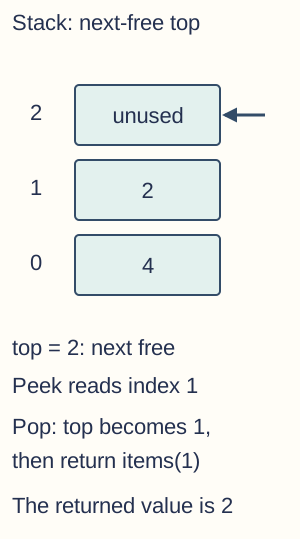
Final state after push 4, push 9, peek, pop, push 2 under the next-free top convention: live values 4 and 2 at indices 0 and 1, top 2. Peek reads index 1. A subsequent pop decrements top to 1 then returns 2; the unused slot is not a live zero value.
Underflow and overflow — Underflow is an invalid removal or inspection when no item is available; bounded-stack overflow is an insertion when no capacity remains. Handle both according to the declared interface, and preserve state on rejected operations. This structure-level overflow is distinct from numeric arithmetic overflow, though both involve exceeding a limit.
Linked stack and uses — A linked stack can keep a head reference as the top: push links a new node before the old head, and pop advances head to its next reference. These local operations avoid shifting all other items, but allocation/references consume resources. A dynamically allocated stack can still exhaust available memory; dynamic does not mean infinite.

Graphs and graph representations

Vertices and edges — A graph models entities as vertices/nodes and relationships as edges/arcs. A transport map can model stations and connections; a dependency graph can model tasks and prerequisite directions. An edge's meaning must be defined: geographical closeness alone is not proof of a route or a prerequisite.
Directed and undirected graphs — An undirected edge represents a symmetric connection, so A–B also connects B–A. A directed edge A→B need not imply B→A, as in one-way travel or a link. State whether self-loops and parallel edges are permitted in the particular model rather than assuming every graph is a simple graph.
Weights and paths — A weighted edge stores a cost such as distance, time or capacity. A path follows adjacent vertices under the permitted directions; its total cost is a sum of relevant edge weights for a suitable additive model. Fewest edges need not mean lowest total weight, and shortest is ambiguous until the optimisation criterion is specified.
Adjacency matrix — For n labelled vertices, a basic adjacency matrix has n by n entries, with row i and column j describing the edge from i to j. An undirected simple graph gives a symmetric matrix. A Boolean matrix can use 1 for present and 0 for absent; a weighted matrix needs an unambiguous no-edge marker if zero-weight edges are allowed.
Adjacency list — An adjacency list stores each vertex's neighbours, optionally alongside edge weights. For a directed graph it commonly lists outgoing neighbours; for an undirected graph each edge is normally represented in both endpoint lists. Include isolated vertices with empty lists if their existence matters, rather than dropping them because they have no edges.
Comparing graph storage — Here V is the number of vertices and E the number of edges; Θ describes a tight growth bound, matching upper and lower scaling. A basic matrix uses Θ(V²) entries and supports direct edge-presence access by indices; a list uses Θ(V + E) space under the usual representation and directly enumerates actual neighbours. Sparse graphs have relatively few edges compared with the possible number and often favour lists. Dense graphs have many of the possible edges; these graphs, or workloads with frequent arbitrary edge queries, may suit matrices. List edge lookup may need a scan unless a different neighbour container is chosen.
Worked representation — For undirected edges A–B and B–C with isolated D, the lists are A:[B], B:[A,C], C:[B], D:[]. The symmetric matrix in A,B,C,D order has ones at AB, BA, BC and CB, with all remaining entries zero for this simple unweighted example. Reordering vertex labels changes row/column positions but not the underlying graph if the key is updated.
The same undirected simple graph as a drawing, a Boolean matrix and adjacency lists. Edges A-B and B-C are represented in both directions; D remains an isolated vertex with an all-zero matrix row/column and empty list. Matrix order is explicitly A,B,C,D.
Graph model limitations — Decide whether weights can be negative, whether edges are directed and what disconnected vertices mean before applying a search or shortest-path algorithm. A matrix's shape alone does not prove an algorithm's assumptions. Graph traversal and shortest-path methods are developed in the algorithms chapter using these representations.

Trees, rooted trees and binary trees

Tree definition — A tree is a connected undirected graph with no cycles; it need not have a designated root. Between any two vertices there is exactly one simple path, a path with no repeated vertex, and a finite tree with n vertices has n−1 edges. An acyclic but disconnected graph is a forest, not one connected tree.
Rooted relationships — A rooted tree designates one vertex as root, creating parent/child relationships. The root has no parent; every other node has one parent along its path from the root. Descendants lie below a node under this chosen orientation, and siblings share a parent. Rooting changes the hierarchy interpretation without adding an extra graph edge.
Leaves, depth and height — A leaf in a rooted tree has no children. Under an edge-count convention, root depth is 0, a child's depth is its parent's depth + 1 and a tree's height is the maximum depth. Other sources count nodes/levels instead; declare the convention rather than treating height 3 and 4 as automatically contradictory without inspecting definitions.
Binary tree — A binary tree is a rooted tree whose nodes each have at most two children, usually distinguished as left and right. It is not necessarily full, complete or balanced, and two is a maximum rather than a requirement for every node. A binary tree can represent an arithmetic expression where internal nodes are operators and leaves operands.
Binary search tree — A binary search tree adds an ordering invariant, such as all keys in a node's left subtree smaller and all in its right subtree larger. Decide how duplicate keys are rejected, counted or placed; an arbitrary binary tree is not automatically searchable using this comparison rule. The invariant concerns entire subtrees, not merely the immediate children.
A rooted binary search tree with keys 8,3,10,1,6. Every key in 8's left subtree is smaller than 8. Under edge-count convention root depth 0 and height 2; leaves 1,6,10. There are five vertices and four edges. This example assumes unique keys and illustrates no balancing algorithm.
Tree representations and performance — A node can hold data and left/right references, using Nothing for an absent child; parallel arrays can instead hold data and child indices with a defined null marker. Balanced search trees can keep path lengths logarithmic, while an unbalanced chain can make search linear. The shape and maintenance rules, not merely the word tree, determine operation costs.

Hash tables, collisions and dictionaries

Key-value mappings — A dictionary associates unique keys with values so a value can be retrieved using its key. Candidate code → score and word → frequency are examples. Different keys can have equal values; key uniqueness does not imply every stored score or frequency is different.
Hash table implementation — A hash table implements a mapping by converting a key through a hash/index rule into a table position or bucket. An example integer index rule is key Mod tableSize for suitable nonnegative keys. The rule should distribute the relevant keys reasonably; a hash is not automatically unique, and hashing is not encryption.
Collisions — A collision occurs when different keys map to the same relevant hash or table position under the stated mapping. With size 7 and index key Mod 7, keys 10 and 17 both map to index 3. A duplicate insertion of the same key is a separate dictionary policy issue: it might update the value or be rejected, rather than being treated as a new distinct key.
Probing and rehashing — A collision can trigger another hash/probe position, such as linear probing (initialIndex + step) Mod tableSize for steps 1,2,… until a suitable slot is found. Some course descriptions call seeking another hash position rehashing; implementations also use rehash to mean rebuilding a table at a new capacity. State which operation is meant instead of assuming those uses are identical.
Worked collision resolution — In a seven-slot table using linear probing, inserting key 10 occupies index 3. Inserting key 17 also begins at 3, compares the stored key, then tries 4 if empty. Looking up 17 must follow the same probe sequence and compare keys; finding any occupied slot at the initial hash is not sufficient evidence of a match.
Deletion and empty markers — In open addressing, deleting a key by marking its slot as never-used empty can break lookup for a later colliding key. A tombstone can mean deleted-but-continue-probing, while a genuinely never-used empty slot can terminate an unsuccessful search under the chosen algorithm. Preserve the distinction, handle a full probe cycle and consider periodic rebuilding.
Seven-slot open-addressed table after inserting 10 at 3, inserting 17 at 4 and deleting 10. Slot 3 is a tombstone, so a 17 lookup beginning at 3 continues to 4 and verifies the key. Marking 3 as never-used empty would incorrectly terminate that lookup.
Load and resizing — Load factor is the number of live entries divided by the relevant table capacity in a simple open-addressed model. Greater occupancy tends to increase probe work, and a policy may resize/rebuild before the table is full. Average expected constant-time access needs assumptions about distribution and occupancy; worst-case lookup can still be linear.
Separate chaining — Another collision strategy keeps multiple entries in a bucket, such as a linked list. Lookup searches that bucket for the actual key, and deletion need not break an open-address probe chain because no such chain is used. Compare the representation's memory and operation rules; do not mix bucket-list deletion with tombstone rules from open addressing.
Dictionary word counts — To count words, normalise according to a declared policy, then for each word add a missing key with count 1 or increment its existing count. For "Red red blue", ignoring case and using spaces as the teaching separator, the mapping is red:2 and blue:1. Real tokenisation needs decisions about punctuation, apostrophes and languages; sorted display order is not inherent in the abstract dictionary.

Vectors as indexed values and mathematical objects

Vector representations — A finite vector is an ordered collection of entries from a specified mathematical field (a number system supporting the required arithmetic, for example the real numbers). An example is u = [2,3] in ℝ². It can be represented by a list, a one-dimensional array or a function mapping index 0→2 and 1→3; an index-keyed dictionary is another representation. The field ℝ contains real values, not unrestricted mixed text and numeric objects.
Order and dimension — A vector's dimension is its number of components in this finite coordinate setting. [2,3] differs from [3,2], and a two-vector does not become a three-vector merely by changing its display. A position vector can be visualised as an arrow from the origin to its coordinate point, while another interpretation might treat entries as measured features rather than spatial coordinates.
Vector addition — Add equal-dimension vectors component by component: [2,3] + [4,−1] = [6,2]. As displacement arrows, addition gives the combined translation; it is not concatenation into a four-element list. Define and enforce compatible dimensions before implementing the operation.
Scalar multiplication — Multiplying a vector by scalar k multiplies each component: 3[2,−1] = [6,−3]. A positive scalar scales in the same direction, a negative scalar reverses direction and zero gives the zero vector. Scaling a position vector can change its distance from the origin; it is not automatically a translation by a fixed vector.
Convex combinations — A convex combination αu + βv requires α ≥ 0, β ≥ 0 and α + β = 1. For u = [2,0], v = [0,4], α = 0.25 and β = 0.75, the result is [0.5,3], on the segment between the endpoints. A general linear combination with negative coefficients or a different sum need not stay on that segment.
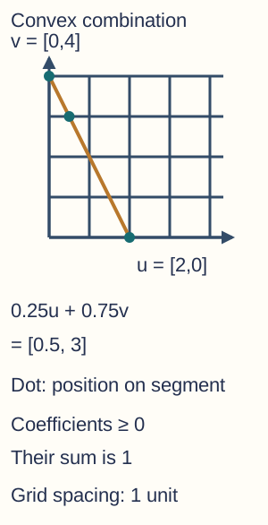
Coordinate example for endpoints u=[2,0] and v=[0,4]. The weighted point 0.25u+0.75v=[0.5,3] lies on their segment. Each square is one coordinate unit. The highlighted segment is a locus of combinations, not an extra vector component or a time trajectory.
Dot product — For compatible real vectors, u·v is the sum of component products: [1,2]·[3,4] = 1×3 + 2×4 = 11. The result is a scalar, not another vector and not componentwise multiplication [3,8]. State the coordinate field and dimension assumptions and include every component once.
Magnitude and angles — The Euclidean magnitude is ‖u‖ = √(u·u). For nonzero u and v, cos θ = (u·v)/(‖u‖‖v‖); use the inverse cosine in the intended angle unit. For [3,0] and [0,4], the dot product is 0 and θ = 90°. The zero vector has no defined direction here, so the angle formula cannot be applied by dividing by its zero magnitude.

Worked vector angle — For u = [1,2] and v = [3,4], ‖u‖ = √5, ‖v‖ = 5 and cos θ = 11/(5√5) ≈ 0.98387. Thus θ ≈ 10.3° rather than 11°. Intermediate rounding and floating-point error can affect a numerical implementation; distinguish a tiny rounding excursion outside [−1,1] from fundamentally incompatible or invalid input.

Dot product and angle fragments — Original VB.NET with Option Strict On, inside the example module. File fragments need System.IO, System.Text and System.Collections.Generic imports as used in the retained source. Work only with deliberate practice files.

Public Function Dot(u() As Double, v() As Double) As Double
    If u.Length <> v.Length Then Throw New ArgumentException("Different dimensions")
    Dim result As Double = 0
    For i As Integer = 0 To u.Length - 1
        result += u(i) * v(i)
    Next
    Return result
End Function
Public Function AngleDegrees(u() As Double, v() As Double) As Double
    Dim uLength As Double = Math.Sqrt(Dot(u, u))
    Dim vLength As Double = Math.Sqrt(Dot(v, v))
    If uLength = 0 OrElse vLength = 0 Then Throw New ArgumentException("Zero-vector angle")
    Dim cosine As Double = Dot(u, v) / (uLength * vLength)
    ' Finite ordinary teaching inputs; clamp only tiny rounding excursions.
    If Double.IsNaN(cosine) OrElse Double.IsInfinity(cosine) OrElse cosine < -1.000000000001 OrElse cosine > 1.000000000001 Then
        Throw New ArithmeticException("Invalid cosine")
    End If
    cosine = Math.Max(-1, Math.Min(1, cosine))
    Return Math.Acos(cosine) * 180 / Math.PI
End Function

Representation versus operation — A dictionary representation of a vector must still preserve the intended index domain, missing-entry policy and order when converting to a list or array. A sparse representation may omit components only under an explicit default-zero convention. The storage choice does not change the mathematical meaning of addition, scaling, convex combination or dot product.

K5CS2 · Data structures, files and vectors