 Mr Kidman's Classroom



Revise the key ideas
Banks, credit and financial decisions
- Saving, investment and intermediation — Saving means income not spent on current consumption; economic investment concerns adding to productive capital rather than every purchase of a financial asset. Banks and other financial institutions connect payment, saving and borrowing decisions, helping resources move between users and periods. Evaluate the terms, risk and purpose. More available credit can support investment without guaranteeing that every financed project is productive or sustainable.
- Banks and deposit creation — A commercial bank can create a matching deposit when it makes a loan; it is not simply passing a fixed stock of existing deposits from one named saver to one borrower. Lending remains constrained by capital, liquidity, credit risk, demand, funding conditions and regulation. Repayment and default also matter. Do not infer that creating deposits permits unlimited costless credit or makes banks indifferent to savers and funding.
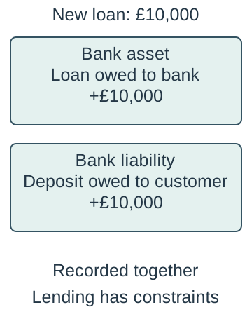
A fictional new £10,000 loan creates a corresponding loan asset and deposit liability on the bank’s balance sheet. The two records are simultaneous counterparts, not a sequence of two independent loans. Actual lending remains constrained by capital, liquidity, risk, funding, demand and regulation. Source: Bank of England: money creation.
- Credit and its purpose — Credit provides purchasing power or permits payment later, with an obligation under agreed terms. A firm may borrow for equipment, a period before customer receipts arrive or an unexpected cost. Distinguish the purpose and duration rather than assuming every loan finances expansion. A useful asset or profitable sale can create a cash-timing need before it produces receipts.
- Interest and borrowing cost — Interest is charged for use of borrowed funds over an agreed period, with the total cost also affected by fees and terms. In an original simple-interest exercise, £10,000 at 6% for one year incurs £600 interest before fees: 10,000 × 0.06. This is a teaching assumption, not a quotation or a complete loan repayment schedule. Compounding or changing balances would require different working.
- Collateral and security — Collateral is an asset offered as security under the borrowing arrangement. It can reduce a lender's potential loss and affect access or terms, but does not guarantee repayment or remove every risk. The borrower may lose the secured asset if relevant conditions for enforcement arise. Distinguish an asset's estimated value from cash available immediately and avoid treating every firm as having acceptable security.
- Creditworthiness and information — Lenders assess the likelihood of repayment using relevant information such as cash flow, commitments, history and the project. A new firm can face uncertainty and limited records even with a promising idea. The lender's information may be incomplete and its judgement fallible. Access depends on terms and conditions as well as the general level of rates; a willing borrower does not automatically obtain any requested amount.
- Risk and liability — Risk concerns possible adverse outcomes and the exposure a decision creates. Liability concerns responsibility for obligations such as debts under the applicable legal arrangement. They are related but not identical. Limited liability does not make a venture risk-free, while an unlimited-liability owner can face consequences beyond the funds initially put into the activity. The later finance chapter develops probability-based risk versus deeper uncertainty.
- Limited and unlimited liability — For a typical UK limited company, the company is legally distinct from its owners and shareholders' exposure is generally limited under the relevant share and legal arrangements. A sole trader is personally responsible for business debts. Guarantees, misconduct and other arrangements can alter exposure, so do not claim that every company owner can never lose personal assets. These are core economic distinctions, not personal legal advice.
Source: GOV.UK: business structures.
- Loans — A loan normally provides an agreed sum with repayment and interest arrangements over a specified term. It can support planned investment when repayments fit expected cash generation, but commitments persist if sales disappoint. Compare term, flexibility, security and total cost with the intended use. A lower stated rate alone does not prove that a particular loan is the best or cheapest overall arrangement.
- Overdrafts — An overdraft permits a bank account to go below zero within agreed arrangements. It can accommodate short-term timing fluctuations, but limits, cost and the possibility of withdrawal create constraints. It is not free permanent capital. Compare the flexibility with the consequences of relying on it for a long-lived investment or a persistent unviable operating deficit.
- Trade credit — Trade credit allows a business to receive inputs and pay the supplier later under agreed terms. It can help bridge the time before sales receipts but creates a payable and may affect discounts or supplier relationships. It is different from a customer paying in advance. A longer payment period can benefit one firm's cash flow while imposing financing pressure on its supplier.
- Equity and venture capital — Share capital raises finance by issuing ownership interests rather than promising the same contractual repayments as a loan. Investors can require returns and influence, and existing ownership can be diluted: issuing new shares can reduce an existing shareholder's percentage ownership and voting power. Venture capital typically involves investors providing equity to selected higher-growth or higher-risk ventures with active expectations about development and eventual exit. It is not an unlimited grant or automatically suitable for every small firm.
- Leasing and access to assets — Leasing provides use of an asset under agreed payments and conditions rather than an immediate outright purchase. It may reduce the initial cash outlay and help access equipment, while total costs, use restrictions and ownership terms matter. Do not assume every lease ends with ownership or that spreading payments makes the resource cheaper overall. Compare the actual agreement and intended period of use.
- Internal and owner finance — Owner savings can finance activity without a new external lender but have an opportunity cost and personal exposure. Retained profit is profit kept in the business, not a guarantee of available cash at that moment. Selling assets can release cash while reducing productive capacity or future flexibility. Internal finance is constrained by what the firm actually has and by its future needs.
- Individual investors and collaborative funding — Individual investors can provide funds through different arrangements, including equity or lending. Online collaborative funding can involve donations, rewards, debt or ownership, with different obligations and risks. Identify which model applies rather than calling all crowdfunding a loan or free finance. A successful campaign can create delivery commitments, platform costs and expectations as well as cash.
- Credit and the wider economy — Credit can support household spending, working capital (funds supporting day-to-day operations before customer receipts arrive) and investment, creating demand and productive opportunities. Excessive or poorly assessed borrowing can increase vulnerability, while a contraction of lending can disrupt viable activity as well as risky projects. Trace effects through spending, repayments and confidence. An economic benefit from access does not imply that expanding every form of credit without limit improves welfare.
Market failure, externalities and intervention
- Markets and social outcomes — A market can coordinate information, incentives and exchange, yet a privately chosen outcome need not make the best use of resources from society's perspective. Market failure concerns a relevant inefficient allocation, not simply any outcome someone dislikes or any firm making a loss. State the failure and mechanism. Distributional concerns can also motivate policy but are not identical to every technical efficiency claim.
- Private, external and social costs — Private costs fall on participants in the relevant transaction; external costs affect third parties without being fully reflected in it. Social cost combines the private and external costs under a consistent definition and period. In an original per-unit exercise, £10 private cost plus £4 external harm gives £14 social cost. Do not add a total annual harm to a per-unit cost without conversion.

Original consistent per-unit example: private cost £10 plus external cost £4 gives social cost £14. The numbers are fictional and do not estimate a real externality. Total and per-unit amounts must not be added without alignment. - Private, external and social benefits — Private benefits accrue to participants while external benefits spill over to third parties not fully captured by the transaction. Social benefit combines the relevant private and external benefits. A training programme can benefit the learner and employer and potentially others through shared knowledge, but identify an actual mechanism. A benefit to the paying customer alone is not an external benefit just because the product is socially approved.
- Production and consumption effects — External effects can arise while producing or consuming a good. Noise from production can affect neighbours; use of a service can create benefits or harm for others. Analyse the particular activity and third party, avoiding a blanket claim that every unit or user has the same effect. The existence, size and distribution of an externality need evidence in real cases.
- Why external costs can distort output — If a decision-maker faces only private costs while some relevant harm falls on others, the private incentive can encourage more activity than is socially efficient. Compare the benefit and cost of an additional unit, not merely whether the total activity has any benefits. A useful good can still be overproduced at the margin. The argument does not imply that eliminating all production is necessarily optimal.
- Why external benefits can distort output — When part of an activity's benefit accrues to others and cannot be captured by the buyer or producer, the private incentive may support less than the socially efficient amount. An additional unit can have social benefit above its resource cost even when the private purchaser declines it. Identify the relevant spillover and constraints rather than assuming every beneficial activity warrants an unlimited subsidy.
- Efficiency at the margin — Marginal means the effect of one additional unit or change. A standard efficiency judgement compares marginal social benefit with marginal social cost: expand while the former exceeds the latter under the model's assumptions. Equality can identify an efficient margin in the appropriate model, not a guarantee of fairness. Comparing total benefits and costs alone does not show whether the current final unit is efficient.
- Policy purpose and baseline — Define the problem, intended change, affected agents and comparison before selecting an intervention. Compare feasible policy with the likely outcome without it and with alternatives, including implementation limits. A declared target is not an achieved result. The relevant question is whether an intervention improves the outcome after its own costs and effects, not whether a perfect solution exists.
- Regulation and legislation — Rules can restrict harmful activity, require standards, change rights or impose responsibilities. A rule needs a clear scope, monitoring and a credible enforcement arrangement. It can directly constrain conduct when price responses are weak, but compliance and administration use resources. A law's existence does not establish full compliance or that all affected firms bear the same cost.
- Indirect taxation — A tax on a harmful activity can raise the private cost or price and reduce activity, depending on supply, demand and enforcement. The amount paid by firms or consumers depends on market responses, not only who legally sends the payment. A rate that matches estimated external harm can be difficult to identify and update. Revenue can fund other activity, but that does not by itself prove the tax corrects the failure efficiently.
- Grants and subsidies — A subsidy can lower relevant costs or support activity with external benefits, while a grant can provide specified financial support. Their effects depend on design, eligibility, demand, capacity and whether activity would have occurred anyway. Funding has an opportunity cost and may be captured without the intended additional benefit. Evaluate the actual mechanism rather than assuming every recipient passes all support to consumers.
- Voluntary agreements — A voluntary agreement seeks changes in behaviour without relying solely on compulsory sanctions. It can use industry knowledge and flexibility, but participation, monitoring, incentives and credibility affect compliance. A firm announcing a target is not evidence of an achieved reduction. Compare the agreement with feasible rules or price incentives, noting the risk that non-participants benefit without contributing.
- Government failure — Government failure occurs when intervention creates a worse resource allocation than the relevant feasible alternative after its effects and costs. A policy being imperfect is not enough to prove that doing nothing would be better. Investigate distorted signals, unintended responses, administration and information gaps. An externality's existence and a policy's failure can coexist; neither proves all markets or all intervention always work badly.
- Signals and unintended consequences — Intervention can change incentives in ways not captured by the initial intention. A subsidy based only on output can encourage low-value production, while a poorly designed restriction can shift activity elsewhere. Identify the actual behavioural channel and who responds. Distortion is not a synonym for every price change: an intentional correction of an externality may improve a previously distorted incentive.
- Administrative cost and information gaps — Designing, monitoring and enforcing a scheme uses resources, and decision-makers may lack reliable information about harm, demand, costs or responses. These limits can cause poorly targeted support or inefficient rules. More measurement can help but also costs time and money. Explain what information matters most and whether a simpler feasible alternative would perform better.
- Evaluating intervention — Judge an actual supplied or fictional policy against effectiveness, cost, equity, incentives, compliance, distribution and time. A short-run reduction may not persist; a firm can adapt or relocate; costs can fall unevenly. State the criterion behind the conclusion and the most important uncertainty. A balanced argument explains mechanisms and evidence rather than automatically giving one unconnected advantage and disadvantage.
Revenue and the behaviour of costs
- Sales volume and revenue — Sales volume counts output sold over a period. For a uniform price, sales revenue equals price multiplied by quantity sold. In an original example, 150 units at £20 produce £3,000 revenue. If different units have different prices, calculate and add the relevant revenues rather than applying one unsuitable price. Production exceeding sales can create stock without generating sales revenue yet.
- Revenue versus receipts — Revenue records sales under the relevant accounting basis, while cash receipts record money actually received. A credit sale can create revenue before payment arrives; an advance can bring cash before the associated activity is completed. State the timing and measure in a question. Treating every sale as immediate cash can conceal a financing need even when the business appears profitable.
- Fixed costs and the time period — Fixed costs do not change with output within the stated period and relevant operating range, such as an agreed premises cost in a simple model. Fixed does not mean unchangeable forever or unaffected by every decision. Expanding to another site can create a step increase. Define the horizon and range before assuming the same fixed-cost figure applies to every possible output.
- Variable and total costs — Variable costs change with output; total cost is total fixed cost plus total variable cost in the defined model. If variable cost per unit is constant at £8 and 150 units are produced, total variable cost is £1,200. With £1,200 fixed costs, total cost is £2,400. Quantity discounts, waste and capacity constraints can make unit variable costs change in practice.
- Average cost — Average cost equals total cost divided by the relevant output. In the original 150-unit example, £2,400 ÷ 150 = £16 per unit. Dividing total fixed cost by output gives average fixed cost; dividing total variable cost gives average variable cost. Keep the same period and output basis. Average cost is not the total cost or necessarily the extra cost of one more unit.
- Spreading fixed cost — When a fixed amount is shared across more output, average fixed cost falls. £1,200 spread across 100 units is £12 each, while across 200 units it is £6 each. This can reduce average total cost if other costs do not rise enough to offset it. Do not infer that producing more always lowers all unit costs or that selling unwanted output automatically raises profit.
- Output, sales and stock assumptions — A simple calculation often assumes all output is sold and ignores changes in stock, but a real firm can produce and sell different quantities. Identify the assumption before combining production costs with sales revenue. Unsold stock uses cash and resources and can deteriorate. The stock's accounting treatment and timing should follow the data given rather than silently assuming its cost is zero.
- Percentage change in performance — Percentage change is the difference divided by the original value, multiplied by 100. In an original example, revenue rising from £2,500 to £3,000 increases by £500 ÷ £2,500 × 100 = 20%. The same £500 rise from £5,000 would be 10%. Report the base, direction and measure, and do not confuse a percentage change with a percentage-point change in a margin.
- Price, volume and revenue interaction — A price reduction increases revenue only if the resulting quantity response more than offsets the lower price over the relevant comparison. In an original example, 100 units at £20 give £2,000; 120 at £18 give £2,160. Revenue rises £160, but profit still depends on costs. The elasticity chapter formalises the relationship rather than assuming that all discounts improve performance.
- Cost drivers and quality — Wages, input prices, productivity, waste, technology, capacity and the required quality can influence costs. A cheaper component can reduce a purchase payment while increasing defects, returns or lost demand. Analyse total relevant consequences rather than identifying cost efficiency with the lowest immediate price. A productivity gain can create different outcomes depending on pay, output decisions and customer response.
- Reading tables and diagrams — Identify units, period, total versus per-unit measures and the assumed output range before extracting a result. A total-cost line and an average-cost curve have different axes and cannot be compared as if they were the same quantity. Diagrams should label what they measure and support a verbal causal explanation. A straight line is an assumption to test, not proof all real costs behave linearly.
- Performance evidence and causality — A fall in average cost after a change may reflect higher output, input prices, quality changes or another influence as well as the proposed improvement. Compare like with like and consider what would have happened otherwise. A table can establish the stated arithmetic without proving its cause. Use actual supplied evidence and qualify wider claims rather than inventing a firm's results.
Contribution, break-even and risk
- Contribution per unit — Contribution per unit equals selling price minus variable cost per unit. In an original model, £20 − £8 = £12. Each sold unit contributes that amount towards fixed costs and, after those are covered, profit. Contribution is not automatically profit per unit because the fixed costs still need to be met. State that the simple model assumes the relevant price and unit variable cost remain constant.
- Total contribution — Total contribution equals contribution per unit multiplied by quantity sold under the uniform assumptions, or total revenue minus total variable cost. At 150 units and £12 each, total contribution is £1,800. Subtract £1,200 fixed costs to obtain £600 model profit. Do not subtract the same variable costs again after already using contribution.
- Break-even condition — Break-even is the output at which total revenue equals total cost and model profit is zero. It is not the point of maximum profit or necessarily immediate cash solvency. Below that quantity, fixed costs are not fully covered under the model; above it, positive contribution can generate profit. The conclusion depends on the price, costs and actual ability to sell the output.
- Calculating break-even output — With positive constant contribution, break-even quantity equals fixed costs divided by contribution per unit. In the original model, £1,200 ÷ £12 = 100 units. State units and the period. A calculation yielding a fraction may need rounding up to the next whole saleable unit to reach at least break-even; do not round down merely because the decimal is small.
- Break-even diagram — Plot quantity per period horizontally and total money amounts vertically. The fixed-cost line is horizontal within the stated range; total cost begins at fixed cost and rises with variable cost; revenue starts at zero in the simple uniform-price model. Their intersection shows break-even. Label the lines and quantity, and distinguish a loss or profit gap at a particular output from the fixed-cost amount.

Original model with price £20, unit variable cost £8 and fixed cost £1,200 per period. TR is total revenue, TC total cost and FC fixed cost. At 100 units, revenue and total cost both equal £2,000. The money axis and quantities are schematic representations of that linear model, not observed data; demand, capacity and constant-price/cost assumptions still need evaluation. - Margin of safety — Margin of safety is actual or forecast sales quantity minus break-even quantity in the same period. At 150 forecast units and 100 break-even, it is 50 units. If expressed relative to forecast sales, 50 ÷ 150 × 100 is about 33.3%; state that denominator. It shows a model buffer against falling sales, not a guarantee that no other risk exists.
- Changing price or costs — With other assumptions unchanged, a higher price or lower unit variable cost raises contribution and lowers break-even; higher fixed cost raises break-even. Explain possible interactions: a higher price may reduce demand, and improved equipment can raise fixed cost while reducing unit variable cost. The calculation alone does not establish which option gives the best realistic outcome.
- Zero or negative contribution — If price equals variable cost per unit, sales do not contribute to positive fixed costs in the simple model, so dividing by zero does not give a meaningful finite break-even quantity. If contribution is negative, more sales worsen the model loss before fixed cost. Do not interpret a negative algebraic quantity as an achievable break-even output. Different products or strategic decisions would require additional analysis.
- Capacity and demand constraints — A calculated break-even quantity can exceed the firm's capacity or plausible demand. In that case, the current plan is not feasible under its assumptions, even if the arithmetic is correct. Compare expected sales, available resources and changes to price or costs. It is not enough to state that the firm should simply sell the required quantity when customers and capacity are constrained.
- Limits of the model — Straight-line break-even assumes a relevant range, known costs, constant unit price and variable cost, and a defined product or stable mix. Real output can change discounts, productivity, step costs, stock and demand. Forecast uncertainty also matters. Use the model to clarify a decision and test assumptions rather than treating its intersection as a certain future result.
- Sensitivity and judgement — Test how a plausible change in an important assumption alters break-even and margin of safety. For example, if price falls from £20 to £18 with unit variable cost £8, contribution becomes £10 and break-even rises from 100 to 120 units at the same fixed cost. This does not predict sales will fall or rise; it isolates the model effect before evaluating demand and other evidence.
Profit, loss and accounting margins
- Profit as incentive and signal — The prospect of profit can attract entry and investment, while persistent losses can encourage exit or change. Outcomes depend on expectations, finance, barriers and adjustment costs. A single profitable period does not guarantee future returns, and an observed loss need not cause immediate closure if the firm expects recovery or pursues other aims. Distinguish a signal from a complete explanation of behaviour.
- Revenue and cost of sales — A simplified statement of comprehensive income begins with revenue and deducts the cost of sales to obtain gross profit. Cost of sales refers to the relevant cost of the goods or services sold under the stated accounting data; it is not automatically every cash payment in the period. Use the supplied categories and avoid subtracting a cost twice through inconsistent classifications.
- Gross profit working — In an original statement, revenue is £100,000 and cost of sales £60,000, so gross profit is £40,000. It is a subtotal before other operating expenses and later stated charges. A positive gross profit alone does not establish an overall profit. Check which stage of the sequence an answer refers to rather than using gross and net interchangeably.
- Operating profit working — Deduct other operating expenses from gross profit to obtain operating profit in the required simple sequence. With £40,000 gross profit and £25,000 other operating expenses, operating profit is £15,000. The classification and period must remain consistent. An operating expense is not necessarily paid in cash at exactly the time its cost is recognised.
- Profit for the year — Following the specification's simplified sequence, deduct the stated interest from operating profit to obtain profit for the year, called net profit in this course's required ratios. £15,000 less £3,000 interest gives £12,000. If a question additionally supplies tax or other adjustments, follow its stated categories rather than assuming this teaching sequence is a complete real company's published accounts.

Original simplified statement using k to mean 1,000: revenue £100,000 less cost of sales £60,000 gives gross profit £40,000; less other operating expenses £25,000 gives operating profit £15,000; less stated interest £3,000 gives £12,000 profit for the year. Additional supplied adjustments would need the question’s treatment. - Gross profit margin — Gross profit margin equals gross profit divided by revenue, multiplied by 100. In the original statement, 40,000 ÷ 100,000 × 100 = 40%. It measures gross profit relative to sales, not the percentage mark-up on cost of sales. A margin can improve while gross profit falls if revenue falls sufficiently, so examine both the ratio and the amounts.
- Operating profit margin — Operating profit margin equals operating profit divided by revenue, multiplied by 100. The example gives 15,000 ÷ 100,000 × 100 = 15%. It can help examine operating performance after other operating expenses, but comparisons need consistent categories, periods and context. It does not identify the cause of a difference or establish the firm's available cash.
- Net profit margin — The required profit-for-the-year margin equals the defined net profit divided by revenue, multiplied by 100. The original £12,000 on £100,000 revenue gives 12%. State which profit measure is used. A fall from 12% to 10% is two percentage points, while the relative reduction is 2 ÷ 12 × 100, about 16.7%; these describe different comparisons.
- Margins and mark-up — A margin uses revenue as the denominator; a mark-up uses the relevant cost base. In an original product example, a £20 price and £15 cost give £5 difference: 5 ÷ 20 × 100 = 25% margin, but 5 ÷ 15 × 100 is about 33.3% mark-up. Identify the cost and profit stage in the context. The two percentages cannot be substituted without changing the meaning.
- Ways of improving profit — A firm can seek more revenue, lower relevant costs or a combination through changes to output, price, quality, promotion, process or product mix. Trace demand and cost consequences rather than assuming any single change raises profit. Cutting quality may reduce repeat sales, while extra promotion may cost more than the contribution it generates. Judge the strategy using context and the period involved.
- Comparing performance — Compare amounts, margins, output, market conditions and the basis of the accounts, not one ratio alone. Different business models can have different sustainable margins and volumes. Inflation, unusual items or changed classifications can affect apparent trends. Explain what a measure reveals and what it leaves unknown, including cash, risk, stakeholder consequences and future demand.
Cash flow, survival and financial evaluation
- Cash flow and cash balance — Cash flow concerns money moving into and out of a business during a period; net cash flow is inflows minus outflows. A cash balance is the stock held at a point in time. A positive balance can coexist with negative net flow, and a profitable firm can run short of cash. Define the period and distinguish a stock from a flow before interpreting a forecast.
- Opening and closing balances — Closing cash balance equals opening balance plus net cash flow under the stated model, and becomes the next period's opening balance if no other adjustment is specified. In an original month, £1,000 opening cash plus £4,000 receipts minus £4,500 payments gives £500 closing cash. Show the sequence and sign; do not treat the receipts alone as the closing balance.
- A second forecast period — If the next month opens with £500, receives £3,000 and pays £4,000, net cash flow is −£1,000 and closing cash is −£500. That forecasts a financing shortfall under the assumptions, not necessarily a realised bank balance or evidence an overdraft is already authorised. Identify when arrangements or changes are needed rather than assuming the firm can simply make every payment.

Original fictional forecast: first-period receipts £4,000 less payments £4,500 give −£500 flow; £1,000 opening cash closes at £500. That opens period two, whose £3,000 receipts less £4,000 payments give −£1,000 flow and −£500 closing cash. This identifies a projected funding gap, not an automatically authorised overdraft. - Credit sales and timing — A sale can generate revenue and eventual profit before a customer pays, while materials and wages may need payment earlier. A cash-flow forecast should reflect the actual collection assumptions, such as a stated delay or proportion paid each month. Do not place all credit sales into immediate receipts unless the question specifies it. A profitable expansion can increase this working-capital pressure.
- Capital purchases and loan receipts — Buying equipment uses cash when paid, while the expense recognised in an accounting period can follow a different basis. Receiving a loan increases cash and creates a repayment obligation; it is not sales revenue or profit merely because money enters the account. Separate financing and operating effects so a positive balance is not mistaken for proof that the underlying business is profitable.
- Forecast purpose — A forecast estimates timing and size of inflows, outflows and balances using explicit assumptions. It can identify a shortfall, support planning and help explain credit needs. It does not guarantee customers pay on time or lenders provide the requested facility. Compare forecasts with actual results and revise material assumptions rather than treating the first estimate as a certain outcome.
- Forecast uncertainty — Sales volume, prices, payment timing, input costs, seasonality and unexpected events can alter cash outcomes. Identify the assumptions with the greatest effect and test plausible changes. A detailed spreadsheet can still be unreliable if the inputs are weak. Distinguish a calculation error from a forecast that was arithmetically correct but based on conditions that did not occur.
- Improving cash inflows — Possible actions include collecting receivables sooner, requesting deposits where appropriate, selling surplus assets or arranging suitable finance. Each has constraints: stricter credit terms may lose sales, deposits create delivery obligations and asset sales can reduce future capacity. Borrowing improves immediate liquidity but adds later commitments. Evaluate a specific proposal rather than treating every inflow as free improvement.
- Managing cash outflows — Negotiating supplier terms, adjusting stock, rescheduling feasible spending or changing operating costs can affect timing and amounts. Delaying payment without agreement can damage relationships and supply; reducing stock too far can interrupt production. Cutting an outflow can also reduce productive benefits. Compare immediate survival with the longer-term implications and actual obligations.
- Credit needs and contingency — Use the largest relevant forecast shortfall and timing to identify a potential facility, allowing for reasonable uncertainty and conditions. A forecast minimum of −£500 suggests at least a £500 gap in that simple model, but not a complete financing recommendation. Consider fees, limits, security and repayment capacity using actual supplied data and centre exercises. No borrowing arrangement is assumed to be approved.
- Profit, liquidity and viability — Profitability concerns the relationship between revenue and costs; liquidity concerns meeting cash obligations when due; longer-term viability includes demand, resources, risk and sustainable financing. These are related but distinct. A loan can relieve a timing problem without fixing persistent losses, while a viable profitable firm may need working capital. Use several measures and trace the mechanism before judging a plan.
- Independent financial judgement — Combine relevant calculations, forecast assumptions, market evidence, financing terms and stakeholder consequences to evaluate an unfamiliar business decision. Explain short and longer-term trade-offs and the evidence that could change the conclusion. Original teaching figures are fictional and simplified. A short quiz samples understanding and arithmetic; complete independent statement, diagram, forecast and extended evaluation tasks need fuller evidence.