AD and the general price level — Aggregate demand is planned spending on domestic final output at each general price level: C + I + G + (X − M). In the AD/AS model label the vertical axis general price level and the horizontal axis real output. A point on AD is not a firm's sales at its own product price. Changes in a non-price determinant shift the curve; a changed general price level generates a movement along a given curve.
Why AD slopes down — A higher general price level can reduce real purchasing power, change money-demand and interest conditions, and weaken relative international competitiveness under the model's assumptions. These mechanisms can reduce desired domestic expenditure. Their strength depends on monetary arrangements, wealth, trade and other conditions. Do not confuse a lower general price level with an automatic increase in every household's nominal income.
Short-run aggregate supply — An upward-sloping SRAS curve represents greater output being supplied at higher general prices with relevant input costs and other influences held suitably fixed. Wage and input-price changes, productivity, disruption and indirect costs can shift it. Distinguish movement along SRAS from a non-price shift. Firms, workers and contracts do not all adjust at the same speed.
Long-run productive capacity — Potential or full-capacity output reflects sustainable production with resources and technology under the stated model. It is not literal nonstop use of every person or machine, and sustainable employment can coexist with job matching and structural change. A vertical LRAS benchmark separates long-run capacity from demand; other AS presentations emphasise varying spare capacity. State the model and horizon rather than treating one curve shape as universal fact.
Output gaps — An output gap compares actual output with estimated potential. A negative gap suggests spare resources relative to that benchmark; a positive gap can indicate demand pressure beyond the sustainable level for a time. Potential output is estimated, uncertain and revisable. A high measured unemployment rate or a single busy firm does not precisely identify the national gap by itself.
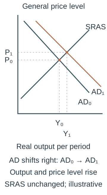
An increase in AD — With an upward-sloping SRAS, a rightward AD shift raises equilibrium real output and the general price level in the simple model. More output can support employment, but labour productivity and hours affect the response. With substantial spare capacity prices may respond less than near capacity. A one-off increase in the price level is not by itself proof of a permanently higher inflation rate.Original schematic: AD shifts right with SRAS unchanged. The new equilibrium has higher real output Y₁ and price level P₁ than Y₀/P₀. The size depends on the slope, capacity and other conditions. A one-off price-level change is distinct from a permanently higher inflation rate; no measured data or calibrated magnitudes are asserted.
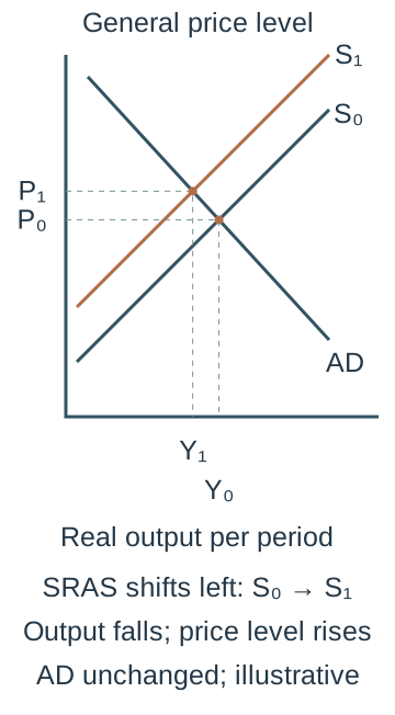
An adverse supply shift — Higher input costs or disruption can move SRAS left, raising the price level and reducing equilibrium output for unchanged AD. This can combine inflation pressure with weaker employment, making demand-only stabilisation difficult. Restricting demand may limit price pressure while worsening activity; supporting demand may protect output while adding price pressure. Explain the trade-off and time horizon.Original schematic: SRAS shifts left/up while AD is unchanged. Output falls from Y₀ to Y₁ and the general price level rises P₀ to P₁. The demand-policy response faces an activity/price-pressure trade-off under these assumptions. Symbols S₀/S₁ denote short-run aggregate supply, not an individual firm's supply.
Capacity improvements — Better infrastructure, skills, capital, technology or market functioning can raise potential output and may also lower short-run unit costs. A rightward supply shift can support more output with less price pressure under stated conditions. Implementation takes time and resources, and demand must support use of the new capability. Extra spending on a project is not itself proof of the intended capacity gain.
Multiplier process — An autonomous increase in spending, meaning spending that rises independently of current income in the model, becomes income for other agents, some of which is spent again on domestic output. Further rounds can make the total output change larger than the initial injection when resources and responses permit. Saving, tax and imports leak spending from successive domestic rounds. This is an expenditure-income mechanism, not a mechanical bank-reserve money multiplier.
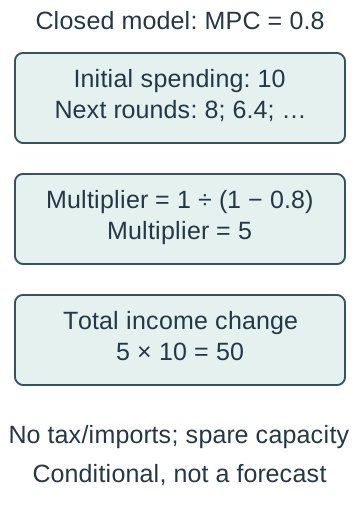
Original multiplier working — In a deliberately simplified closed model without taxes or imports, a constant marginal propensity to consume of 0.8 means that 80% of each additional unit of income is spent on consumption. It gives multiplier 1/(1 − 0.8) = 5. An autonomous spending increase of 10 can then raise equilibrium income by 50. The rounds 10 + 8 + 6.4 + … converge to 50 under the assumptions. This is a model result, not a forecast for an actual UK project.Original closed model without taxes or imports and with constant MPC = 0.8: multiplier 1/(1−0.8)=5. An autonomous 10 injection generates 10+8+6.4+…=50 under the model's equilibrium and supply assumptions. It is not a forecast or a mechanical bank-reserve multiplier.
Open-economy and capacity limits — Taxes, imports, changing saving, credit constraints, confidence, interest rates and supply bottlenecks affect the multiplier. In a simple proportional-leakage formulation it is 1 divided by the marginal propensity to withdraw, the fraction of additional income going into saving, tax or imports under the stated model. For a total withdrawal fraction of 0.25, the model multiplier is 1 ÷ 0.25 = 4. Crowding out or import-intensive spending can reduce the domestic effect. Full capacity can turn extra nominal demand mainly into prices rather than the predicted real-output gain.
Using the model critically — Compare equilibria on fully labelled curves, identify the non-price cause of each shift and explain the causal route to output, prices and employment. Consider simultaneous demand and supply shifts and uncertainty about their relative sizes. Do not label a policy successful merely because a curve was moved on a schematic graph. Test the predictions against dated evidence, distribution and feasible alternatives.
Fiscal and monetary demand policies
Fiscal versus monetary policy — Fiscal policy changes government spending and taxation; monetary policy changes central-bank instruments affecting monetary and financial conditions. They have different authorities, channels, lags and distributional effects, although they interact. A government transfer is not itself a direct output purchase in G, but can affect later consumption. Classify the actual action before applying an AD shift.
Direct and indirect taxes — Direct taxes are levied on relevant income or wealth bases; indirect taxes apply to transactions or expenditure under their rules. Tax changes alter disposable income, costs, relative prices or incentives through different channels. The person paying formally is not necessarily the person bearing the final burden. Specify the base, rate and behavioural response rather than assuming all tax cuts have an identical multiplier.
Government spending choices — Purchases of services, infrastructure or other output can support demand directly, with differing domestic content, timing and capacity effects. A well-chosen investment may improve long-run supply too, while poor design wastes scarce resources. Compare ready-to-deliver support with projects needing lengthy planning. Funding and maintenance matter beyond the initial announcement.
Expansionary and contractionary fiscal measures — Higher spending or lower taxes can support AD; lower spending or higher taxes can restrain it relative to the alternative. Actual net effects depend on recipients' spending, imports, confidence, financing and monetary responses. A larger recorded deficit can arise automatically in a downturn without new discretionary stimulus. Separate the policy decision from cyclical changes in receipts and benefits.
Borrowing and crowding out — Financing a deficit can affect debt obligations, interest costs, confidence and resources available elsewhere. Crowding out can occur through interest or capacity pressures under some conditions; with idle resources and weak private demand, spending may instead support private investment. The effect is not fixed by the word borrowing. Compare the use of funds, horizon and plausible counterfactual.
Policy rates and transmission — The MPC's Bank Rate decision influences wider borrowing and saving rates, credit conditions, asset prices, exchange rates and expectations. Higher rates can restrain spending and inflation pressure; lower rates can support demand when transmission works. Fixed contracts, credit risk, confidence and different household positions create uneven effects. Commercial lenders set their own relevant rates and do not all change them by an identical amount.
Investment, jobs and inflation — Lower financing costs can make some investments more attractive, but expected sales, capacity, risk and access to credit also matter. Stronger demand can support jobs where firms can expand. Close to capacity, extra spending creates more inflation pressure and imports; supply shocks complicate the trade-off. Trace the conditions rather than claiming a rate cut guarantees productive investment.
Quantitative easing — QE purchases assets, especially government bonds, using newly created central-bank reserves through the banking system. It aims to ease financial conditions and support spending through asset prices, yields, portfolios and expectations. It is not free wealth given to banks, direct household cash distribution or a guarantee of proportional new lending. The MPC decides its use within monetary policy; QE changes the composition and size of balance sheets. Bank of England explanation of QE.
Bonds, yields and QE — A bond is a tradable debt claim promising specified payments. For a simple fixed-payment bond, a higher purchase price corresponds to a lower yield, other terms unchanged. For example, a fixed annual payment of 5 gives a current yield of 5% on a price of 100 but 4% on 125; this payment-to-price ratio leaves aside redemption gains or losses. Asset purchases can lower yields and affect other financing costs through portfolio adjustment. Prices, expectations, liquidity and risk premia can complicate actual market responses. Buying an existing bond is a financial transaction, not itself new government spending on domestic output.
Quantitative tightening — QT reduces the relevant asset holdings through maturing assets not being replaced and/or sales under the stated programme. Its effects depend on market conditions, expected future policy and interaction with Bank Rate. It is not simply the identical reverse of QE in every circumstance. Do not infer the current pace or direction of policy from a generic explanation of the tool.
Policy lags — Recognition, decision, implementation and transmission all take time. Tax administration, planning, contract resets, investment delivery and expectations create different lags across instruments and agents. A policy based on revised or delayed data may arrive after conditions change. Compare speed and reversibility with persistence and the risk of overshooting.
Demand-policy evaluation — Assess initial spare capacity, shock type, confidence, financing, exchange rates, import content and distribution. Use success criteria for real activity, inflation, employment, sustainability and welfare, rather than only the size of the instrument. A policy can benefit indebted households differently from savers or firms with imported inputs. Justify conditions and compare a feasible mix of responses.
Supply-side choices and evaluating a policy mix
Market-based supply measures — Competition, entry reform, suitable tax incentives and labour-market flexibility can improve allocation, effort or investment where the identified mechanism operates. Effects depend on opportunities, information, bargaining and enforcement. Removing a rule can reduce unnecessary cost or remove valuable protection, so identify the actual distortion. A policy's market-based label does not guarantee greater welfare.
Interventionist supply measures — Public education, training, infrastructure, research support or targeted coordination can address skills, finance or external-benefit constraints. Quality, access, targeting and complementary investment determine whether productive capacity improves. Funding has opportunity costs and benefits can take years. Judge additional outcomes rather than expenditure or enrolment alone.
Incentives and labour reform — Tax and benefit design, job information, mobility support and employment rules affect decisions under different constraints. Lower marginal deductions may increase the reward to extra work, while childcare, health and vacancies affect what is possible. Flexibility can improve matching or increase insecurity depending on the arrangement. Assess effects on different workers and employers rather than treating labour as homogeneous.
Competition and investment — Credible entry and rivalry can encourage innovation, efficient costs and customer responsiveness. Some scale economies or temporary returns support investment, so the aim is effective competition rather than the largest possible number of firms. Changes in network access or information may be more relevant than ownership alone. Compare price, quality, productivity and dynamic capability over a suitable horizon.
Skills and infrastructure — Training can improve capabilities and transport or digital investment can reduce coordination and mobility barriers. Poor matching, low quality, congestion or maintenance failure can weaken benefits. A project can increase AD during construction and AS later if effective, with distinct time paths. Diagram and explain both mechanisms without assuming every funded project succeeds.
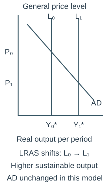
Supply-side diagrams and qualifications — A rightward LRAS shift represents a higher estimated sustainable output; a rightward SRAS shift represents improved short-run supply conditions. A policy may influence both, but state why and when. The final price-level/output result also depends on AD and other shocks. Do not move AD simply because the policy has a favourable name or equate an LRAS label with measured success.Original vertical-LRAS benchmark: productive capacity expands from L₀ at Y₀* to L₁ at Y₁*. With AD unchanged in this long-run comparison, the new equilibrium has more real output and a lower price level. Implementation demand, SRAS adjustment, other shocks and uncertainty about potential output require separate analysis.
Objectives and conflicts — Growth, inflation, employment, distribution, external sustainability, fiscal viability and environmental quality can reinforce or conflict with one another under particular conditions. Demand restraint may lower price pressure while weakening employment; a productive investment can ease a longer-run trade-off while using resources now. The relationship is conditional on shocks, capacity, expectations and implementation. Explain which agents and horizons drive the judgement.
Criteria and evidence — Specify a measurable baseline, appropriate indicator, expected timing and realistic alternative before evaluating effectiveness. Distinguish nominal from real change, level from rate, total from per-head and intention from additional outcome. Use dated data vintages and uncertainty intervals where available. A correlation after a policy is not sufficient proof of its causal effect.
Comparing policy mixes — Choose instruments suited to the diagnosed demand, supply, information or financial problem, considering coordination and conflicting effects. Temporary support can protect viable activity while longer-term measures address capacity, but targeting and financing remain difficult. Test sensitivity to assumptions and identify who may lose or be excluded. A recommendation should state what evidence would reverse it rather than claim a universal best policy.
Risk, uncertainty, insurance and forward markets
Risk and uncertainty — Risk concerns outcomes whose probabilities can be estimated usefully under a stated model; uncertainty concerns outcomes or probabilities not known reliably. The boundary is practical rather than perfectly sharp. A historical frequency may be a poor guide after structural change. Use scenarios, buffers and sensitivity as well as expected values, and do not turn a numerical estimate into certainty.
Economic shocks — Unexpected demand, supply, political, technological or financial changes can alter revenue, cost and financing together. Exposure and ability to adapt determine the effect on a particular agent. A shock helpful to one exporter may harm an importer or borrower. Distinguish the source, transmission and response rather than calling every disappointing outcome an unforeseeable shock.
Original expected-value example — A fictional proposal gives net payoff 40 with probability 0.6 and net payoff −20 with probability 0.4, yielding expected payoff 0.6×40 + 0.4×(−20) = 16. The expected value is a probability-weighted average, not a payoff guaranteed to occur. Cash constraints, downside size, correlation and decision makers' preferences can make two equal expected values very different choices.Original probability-weighted payoff 0.6×40+0.4×(−20)=16. Only 40 or −20 occurs in this two-outcome model; 16 is an average, not a guaranteed realised amount. Downside, liquidity, correlation and reliability of probabilities matter.
Exchange-rate exposure — A business expecting foreign-currency receipts or payments faces changes in their home-currency value. Net exposure depends on matching inflows and outflows, timing, prices and contracts, not gross foreign sales alone. Natural hedging can match currency costs and receipts but may be incomplete. Separate operating, financing and asset exposures when evaluating a shock.
Forward contracts — A currency forward agrees a future exchange on specified terms, reducing uncertainty over that transaction's conversion rate. It can protect against an adverse movement while giving up a favourable movement relative to the locked rate. Counterparty, volume, timing and other business risks remain. A forward fixes a contractual price, not the future spot market or the firm's overall profit.
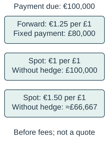
Original forward illustration — A fictional importer must pay 100,000 euros in three months and locks a forward rate of 1.25 euros per pound, fixing the stated payment at £80,000 before fees. At a later spot rate of 1.00 it would otherwise cost £100,000; at 1.50 about £66,667. The hedge removes this conversion uncertainty but can look costly relative to a favourable spot outcome. This is an illustration, not a trading recommendation or quote.Original illustrative importer: 100,000 euros divided by 1.25 euros per pound fixes £80,000 before fees. Spot alternatives 1.00 and 1.50 would imply £100,000 and about £66,667 without the hedge. The forward removes this conversion uncertainty, not all business risk or the possibility of foregoing a favourable movement.
Insurance and business continuity — Insurance transfers specified financial consequences of covered events in exchange for a premium under contract terms. It does not prevent every event or cover every loss, and exclusions, excesses (the part of a claim the policyholder must meet), limits and claims conditions matter. Prevention, diversification, reserves and continuity planning can complement it. Evaluate retained risk, affordability and operational recovery rather than treating insurance as guaranteed full compensation.
Information and insurance incentives — Insurers assess risk and price coverage using relevant information, while policyholders may know more about their exposure or change behaviour after cover. Adverse selection concerns who seeks cover given hidden risk; moral hazard concerns changed incentives after protection or expected support. Monitoring, excesses and prevention conditions can help but have costs. These are analytical mechanisms, not accusations that every claimant acts dishonestly.
Financial services, markets and the central bank
Mobilising savings and finance — Financial institutions connect saving, borrowing, investment and risk management through different instruments and markets. Banks also create deposits when lending; they are not constrained to relend a fixed stock of prior household deposits one for one. Capital, liquidity, funding, regulation, credit risk and demand constrain lending. Distinguish saving's financing role from a mechanical reserve multiplier story. Bank of England explanation of deposit creation and constraints.
Working capital and investment lending — Firms may borrow to bridge the timing between inputs, production and customer receipts as well as to finance longer-lived assets. A profitable firm can face a liquidity shortage, while borrowing cannot make an unviable activity profitable by itself. Match maturity, repayment, security and risk to the purpose. A loan receipt is financing, not operating sales revenue.
Lending to individuals — Mortgages and other credit can bring spending forward or finance an asset, creating repayment obligations and exposure to income, rates and asset values. Terms, affordability and security matter for borrowers and lenders. Household borrowing can support demand while raising vulnerability if obligations outgrow resources. Economic analysis of the mechanism is distinct from advice to take a particular financial product.
Payments and exchange — Payment systems, deposits and settlement services enable transactions and reduce the need for direct barter. Reliability, access, fraud prevention and liquidity support confidence and economic activity. A disruption can harm otherwise viable firms through delayed receipts and wages. The financial sector's role is broader than lending or stock-market trading alone.
Assessing credit risk — Lenders assess the risk of non-payment using income or cash flow, existing obligations, security, purpose and plausible shocks. Collateral can reduce losses but its value can fall at the same time as borrowers' repayment capacity. A statistical score or optimistic past default rate does not eliminate uncertainty. The specification's creditor-risk wording is taught as assessment of lending and repayment exposure, not a claim that every lender is risk-free.
Currency, commodity and equity markets — Forward currency and commodity markets can help users manage specified future prices or receipts, while also permitting speculation and involving counterparty risk (the other party failing to meet its promise) or basis risk (the hedging instrument's price not moving exactly with the exposure it is intended to cover). Equity markets allow ownership claims to be issued and traded, supporting finance, liquidity and price discovery. Buying an existing share transfers ownership and does not itself hand new funds to the issuer. Market liquidity and prices can change sharply under stress.
The MPC's monetary role — The Monetary Policy Committee decides Bank Rate and relevant monetary tools to pursue the government's inflation target, with the broader objectives subject to price stability under its remit. Its decisions affect financial conditions with lags and uncertainty. It does not choose every commercial lending rate or oversee every individual bank's daily risks. Distinguish monetary demand management from financial-system resilience. Bank of England monetary framework.
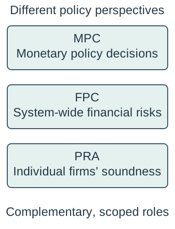
FPC and prudential supervision — The Financial Policy Committee identifies and acts on risks to the stability of the financial system as a whole. The Prudential Regulation Authority focuses on the safety and soundness of individual firms within its scope; other bodies also have relevant roles. System-wide and firm-level perspectives complement one another. Do not treat the FPC as the committee setting Bank Rate or as the sole regulator of every financial activity.Distinct complementary perspectives: MPC makes monetary decisions; FPC addresses system-wide financial risks; PRA focuses on individual firms' safety and soundness within its scope. Other authorities and functions also matter. The FPC is not the Bank Rate committee and these boxes are not a complete institutional chart.Bank of England distinction between FPC and PRA roles.
Banker to banks and last-resort liquidity — Central-bank accounts and operations support settlement and liquidity in the banking system. Last-resort support can address exceptional liquidity stress under relevant conditions and safeguard stability, but is not a guarantee that every insolvent institution or investor will be rescued without loss. Liquidity is ability to meet payments when due; solvency concerns assets and obligations under the relevant valuation. Public-risk and incentive questions require careful design. Bank of England account of settlement and liquidity operations.
Financial crisis, incentives and regulation
The global financial crisis — The 2007–09 crisis involved interacting weaknesses in credit, housing and funding markets, leverage, risk assessment and financial institutions. US sub-prime mortgage losses were important, but do not reduce the crisis to one borrower group or a single event. International exposures and confidence transmitted stress. The Bank of England's dated timeline records Lehman Brothers' collapse on 15 September 2008 as a major intensification, not the sole beginning. Bank of England crisis timeline, published 2018.
Sub-prime mortgages and risk transfer — Sub-prime lending involved borrowers with weaker credit profiles under the relevant market definitions. Packaging loans into securities could spread risk, but complexity, incentives and correlated housing losses made risk hard to assess. Transfer or a high rating did not eliminate the underlying repayment risk. Falling collateral values could coincide with defaults, weakening apparently protective assumptions.
Leverage and short-term funding — Leverage means using borrowing relative to owners' equity, and high leverage magnifies gains and losses relative to that equity. A simplified institution with assets of 100 funded by debt of 90 and equity of 10 loses all that equity if its assets fall by 10 while its debt stays unchanged. Funding long-lived or illiquid assets with short-term borrowing can create refinancing pressure when confidence falls. An institution can face a run or liquidity shortage before every asset suffers a final loss. Distinguish capital buffers absorbing losses from liquidity resources meeting payments, while recognising stress can connect the two.
Bubbles and speculation — Asset prices can rise on expectations of further resale gains, easier credit or overly optimistic future income, creating vulnerability if beliefs reverse. A price rise alone does not prove a bubble; compare fundamentals and uncertainty. When prices fall, collateral, spending and lending can weaken together. Speculation can sometimes support liquidity or price discovery, so identify the destabilising mechanism rather than using the label as a complete explanation.
Moral hazard and too big to fail — If managers or investors expect public support because failure could damage the system, they may take risks whose full downside they do not bear. This is a moral-hazard concern, not proof that all support is unnecessary during a crisis. Authorities must balance immediate stability with future incentives and public exposure. Credible loss allocation, resolution and supervision can help reduce the trade-off.
Organisational culture and incentives — Rewards tied to short-run sales or reported returns can encourage weak underwriting, concealed risk or excessive leverage when accountability is poor. Challenge, governance, risk systems and long-term incentives affect behaviour. A written code is insufficient if actual rewards contradict it. Examine institutions and incentives without assuming every employee had the same information or intent.
Credit contraction and the real economy — Losses, funding stress and uncertainty can lead lenders to tighten credit, affecting working capital, consumption, investment and employment. Lower activity can create further defaults and weaker collateral, reinforcing financial stress. Viable firms can suffer from unavailable finance even when their products remain useful. Trace the feedback rather than treating finance as isolated from households, firms and public budgets.
Government and household effects — Crisis can reduce tax receipts, increase support needs and expose public funds through stabilisation measures. Households can face unemployment, asset losses, repossession or weaker savings returns, with effects varying widely. Gross support commitments, realised fiscal costs and later recoveries are different measures. Evaluate the alternative of uncontrolled failure as well as the cost and distribution of intervention.
Regulation and resilience — Capital and liquidity requirements, stress testing, supervision, governance and resolution arrangements (plans for managing a failing institution and allocating its losses) can reduce fragility and improve loss absorption. They involve implementation, information and possible financing costs, and cannot guarantee no future crisis. Regulation should consider interconnectedness and activity moving outside its scope. Compare resilience, credit access, incentives and systemic spillovers with a realistic alternative rather than claiming either all regulation or no regulation ensures stability.
Evidence and final judgement — Use dated primary evidence, appropriate accounts and clearly labelled scenarios to assess financial or macroeconomic policy. Separate the shock from amplification, emergency response from long-run incentives, and financial transfers from real resource effects. State uncertainty and compare outcomes for affected groups over time. A defensible judgement identifies conditions, limits and evidence that could change it; it is not a prediction or personal investment recommendation.
Test yourself
50 questions · Random sets of 10. These quick checks support revision; practise longer explanations and justified judgements too.
 Mr Kidman's Classroom