What an algorithm specifies — An algorithm is a finite, unambiguous procedure for solving a defined problem from permitted inputs. Identify the input, the state that changes, the repeated instructions, the stopping condition and the output. A worked example shows execution on that input; it does not by itself prove the procedure works on every allowed input.
Assignment updates state — An instruction x ← x + 2 replaces the stored value of x by two more than its current value. It is not an algebraic equation claiming x equals itself plus two. If x starts at 3, successive applications give 5, 7 and 9. Record the current values after each instruction in their stated order.
Order of assignment matters — With a = 2 and b = 5, the instructions a ← b then b ← a leave both equal to 5, because the second reads the updated a. To swap values, store one original value in a temporary variable: t ← a, a ← b, b ← t. Simultaneous assignments must be explicitly specified.
Flowchart symbols and branches — A flowchart uses an input/output stage, process boxes, decision diamonds and directed flow arrows to express a procedure. Follow the labelled true/false or yes/no branch at each test. A loop returns to an earlier stage; do not infer that a box is performed only once because it appears once on the page.
Pre-test versus post-test loops — A loop testing a condition before the body may execute zero times; a loop testing after the body executes at least once. With x = 5 and a pre-test while x < 5, adding 1 is never executed. A repeat-until version could update x to 6 before testing. Trace the actual location and sense of the condition.
A trace with a boundary — Start n = 1, s = 0. While n ≤ 4, set s ← s + n and then n ← n + 1. The states after the body are (s,n) = (1,2), (3,3), (6,4), (10,5), then the loop stops. The output s = 10 includes 4 because the test used ≤, not <.
Checking termination — An algorithm needs a reachable stopping condition for its allowed inputs. If a loop increases x by 2 from an odd initial value and stops only at x = 10, it may never reach equality. Replace an inappropriate equality test or restrict inputs only if the problem authorises that change; when tracing a supplied procedure, report the limitation.
Problem size and operation count — Choose a size parameter n, such as the number of items in a list or vertices in a network. Count the relevant basic operations as a function of n before comparing efficiency. Runtime also depends on implementation and hardware; an order statement describes growth rather than an exact duration.
Order of an algorithm — An operation count such as 3n² + 7n + 4 has quadratic order, written O(n²), because the n² term dominates for large n. Constant multipliers and lower-order terms do not change this order. Doubling n approximately quadruples the dominant work, but not necessarily the exact finite count.
Common growth rates — Constant, logarithmic, linear, quadratic, cubic and exponential growth differ greatly for large inputs. If order is O(n³), tripling size multiplies the dominant work by 27. If work is proportional to 2ⁿ, increasing n by 1 doubles it; doubling n multiplies it by 2ⁿ, not by 2.
Nested loops — If an outer loop runs n times and an independent inner loop also runs n times per outer step, total inner operations are n². If the inner loop runs i times on outer step i, the count is 1 + 2 + … + n = n(n + 1)/2, still quadratic. Sequential linear loops add to linear order rather than multiply.
Correctness versus efficiency — A fast procedure may be incorrect, and a correct procedure may be inefficient. An exact algorithm is designed to return the required optimum; a heuristic can give a useful feasible answer (one meeting the constraints) without proving optimality (that it is the best possible). Compare results with a bound or independent argument before claiming the best possible solution.
Bubble sort
Adjacent comparisons — To sort ascending, scan adjacent items from left to right and swap a pair when the left item is larger. After a full pass the largest item in the scanned unsorted region reaches its right-hand final position. Record swaps in execution order; comparing each item once with the first item is not bubble sort.
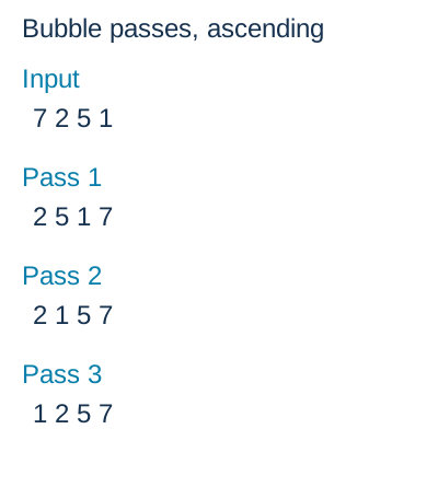
A first pass — For [7,2,5,1], compare 7 and 2 to obtain [2,7,5,1], then 7 and 5 to obtain [2,5,7,1], then 7 and 1 to obtain [2,5,1,7]. This is the end of pass 1, not the fully sorted list. The 7 is now fixed.
Further passes — Scanning the remaining first three entries gives [2,1,5,7] at the end of pass 2. The final comparison of 2 and 1 gives [1,2,5,7]. Reducing the scanned region avoids rechecking the fixed suffix. A no-swap pass is also a valid early stopping certificate for the scanned unsorted region.The states follow left-to-right adjacent comparisons with a shrinking unsorted region. The rightmost 7 is fixed after the first pass and 5 after the second; the final comparison places 1 and 2. The figure records end-of-pass states, while the notes show individual first-pass swaps.
Descending and repeated values — For descending order, reverse the comparison test and swap when the left item is smaller. Equal items need not swap. Keep duplicate values as separate items; sorting does not remove them. If the stated algorithm fixes the pass direction or stopping rule, preserve it in the trace.
Bubble-sort work — The usual shrinking-region worst-case comparison count is (n − 1) + (n − 2) + … + 1 = n(n − 1)/2, so its worst-case order is O(n²). With a no-swap early exit, an already sorted list can be checked in n − 1 comparisons, giving a linear best case for that implementation.
Quick sort and pivots
Divide using a pivot — For ascending quick sort, select a pivot, partition the remaining items into those smaller and those larger, retain the pivot in its final relative position, then recursively sort the sublists: apply the same procedure to each smaller list until it has at most one item. No item may be lost during partitioning. With equal items, use a consistent stated equality rule and retain every copy.
Edexcel's middle-item convention — The pivot is the middle item of the current list: position (n + 1)/2 if n is odd and (n + 2)/2 if n is even, numbering from 1. Thus a list of six items uses its fourth item, not its third; a list of four uses its third. Apply the rule separately to every current sublist.
A partitioned example — For [8,3,7,2,6,1], n = 6 gives pivot 2 at position 4. Keeping the relative scan order in each partition yields [1] | 2 | [8,3,7,6]. The right sublist has four items, so its pivot is 7 at position 3, producing [3,6] | 7 | [8]. The [3,6] pivot is 6, leaving the final order [1,2,3,6,7,8].Brackets identify the first selected pivot in the input and then the current sublists. The six-item list uses its fourth item 2; the four-item right sublist uses its third item 7. The two-item sublist 3,6 uses 6 as pivot before completion. These are partition stages rather than adjacent-swap passes.
Show sublists and fixed pivots — A useful trace separates unsorted sublists from pivots already placed and lists every chosen pivot at each stage. A partition stage is not a sequence of adjacent swaps. Follow the requested number of passes or stages; a final sorted list alone cannot demonstrate the stated pivot rule.
Quick-sort efficiency — With balanced partitions, a level examines O(n) items and there are O(log n) levels, giving typical O(n log n) work. Very unbalanced partitions can lead to quadratic worst-case work. Choosing the middle position is not the same as choosing the median value, so it does not guarantee balanced partitions.
Packing items and assessing bounds
The bin-packing model — Allocate items of given sizes into bins of common capacity C without splitting an item and without exceeding C in any bin. A typical objective is to minimise the number of bins. State units consistently and check that each item individually fits; otherwise the stated packing model is infeasible.
The volume lower bound — If item sizes sum to S, any packing uses at least ceil(S/C) bins, where ceil means round upwards to the next integer (leaving an integer unchanged), since fewer bins cannot hold the total amount. This is a lower bound, not always an achievable count: three items of size 6 in bins of capacity 10 need three bins even though ceil(18/10) = 2.
First fit — Process items in the given order and place each into the first existing bin with sufficient remaining capacity; open a new bin only when none fits. For capacity 10 and items [6,5,4,5], the bins become [6,4] and [5,5]. Searching starts again from the first bin for every new item.
Next fit — Only try the current open bin. If the next item does not fit, close that bin permanently and open the next. For capacity 10 and [6,5,4,5], the result is [6], [5,4], [5]: three bins. The later item 4 cannot return to the closed first bin in this algorithm.Bar widths are proportional to item sizes in equal capacity 10 bins. First fit reuses the first bin for the later 4 and achieves the volume lower bound 2. Next fit has already closed its first bin when 4 arrives, so it produces 6;5+4;5 in three bins.
First fit decreasing — Sort sizes into descending order, then apply first fit to that order. For capacity 10 and [4,4,6,6], ordinary first fit gives [4,4], [6], [6], while first fit decreasing gives [6,4], [6,4]. The preprocessing changes the order; do not apply it when ordinary first fit on the supplied order is requested.
Algorithm result versus optimum — A heuristic packing using B bins gives an upper bound B on the minimum number required. If it matches a valid lower bound L, then L ≤ optimum ≤ B forces optimality. With [6,5,4,5], first fit uses 2 and the volume lower bound is 2, proving it optimal; next fit's 3-bin result is not.
Compare unused capacity — For B equal-capacity bins with total item size S, total unused capacity is BC − S. Its distribution between bins matters for whether later items fit. Two packings can have the same total unused space but different remaining space in individual bins; do not combine fragments across bins to fit one indivisible item.
Practical limitations and communication — Real packing may require shape, weight, compatibility or arrival constraints absent from the one-dimensional model. Give the full item allocation, not merely the bin count, verify capacity and every item exactly once, and distinguish a heuristic outcome from a demonstrated optimum. For flowcharts and sorts, show enough intermediate states to verify the requested algorithm.
Test yourself
50 questions · Random sets of 10. These quick checks support revision; practise longer explanations and justified judgements too.
 Mr Kidman's Classroom