What a differential equation specifies — A differential equation relates an unknown function to one or more of its derivatives. Its order is the highest derivative present. A first-order general solution normally contains one arbitrary constant; a second-order general solution normally contains two. An equation alone describes a family, while suitable initial conditions select a particular member.
Recognising the first-order linear form — An equation y′ + P(x)y = Q(x) is linear in the dependent function y and its first derivative. Divide by a nonzero leading coefficient first, stating any excluded inputs. Terms such as y² or yy′ make the equation nonlinear and do not fit this integrating-factor rule directly.
The integrating factor — Choose μ(x) = e∫ P(x) dx on a valid interval. Multiplying the equation by μ makes its left side μy′ + μPy = (μy)′ because μ′ = Pμ. Therefore μy = ∫μQ dx + C. A nonzero constant multiplier in μ is immaterial; the solution's arbitrary constant absorbs it.
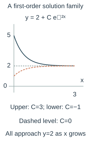
A constant-coefficient first-order example — For y′ + 2y = 4, μ = e²ˣ, so (e²ˣy)′ = 4e²ˣ. Integration gives y = 2 + Ce⁻²ˣ. The constant solution y = 2 is included when C = 0. Differentiating the family and substituting verifies the equation for every real x.
A particular member and its shape — For that equation with y(0) = 5, C = 3, giving y = 2 + 3e⁻²ˣ. As x increases from zero, it decreases toward the equilibrium level two without crossing it. A family sketch should show different C values above, below and at the equilibrium; one graph does not represent every initial condition.Three members of y=2+Ce⁻²ˣ show C=3 above equilibrium,C=−1 below and C=0 at the dashed level two. The displayed interval is 0≤x≤3. Both nonconstant members approach the equilibrium as x increases without crossing it; the curve chosen by y(0)=5 is the upper solid member.
A variable-coefficient example — For y′ + (2/x)y = x on x > 0, μ = e2 ln x = x². Then (x²y)′ = x³, giving y = x²/4 + C/x². The restriction x > 0 was declared before using ln x. The original equation is undefined at zero even if one selected expression happens to have a removable-looking term.
Standard form before integration — For xy′ + 2y = x² with x > 0, divide by x to get the previous equation. Using P = 2 before division would produce the wrong integrating factor e²ˣ instead of x². Match the coefficient of y′ to one before reading P and Q.
Initial conditions and constants — Apply conditions to the complete integrated solution, not only to the homogeneous part (the solution of the equation with zero on its right-hand side). A condition at an excluded singular input is not automatically a valid initial-value problem for the original equation. State the interval of the solution and check both the equation and the specified initial value.
Why constants cannot be discarded — Indefinite integration introduces a constant even when an integrating factor has been chosen conveniently. Dividing μy = H(x) + C by μ gives y = H/μ + C/μ, not H/μ + C unless μ is constant. The x-dependent homogeneous contribution distinguishes the full family.
Second-order linear equations and particular integrals
The homogeneous constant-coefficient equation — For y″ + ay′ + by = 0 with real constants a,b, try y = eᵐˣ. Since eᵐˣ is nonzero, substitution gives the auxiliary equation m² + am + b = 0. Its roots determine the complementary function: the general solution of this homogeneous equation. The independent variable x is distinct from displacement x(t) used later in motion models.
Two distinct real roots — If the auxiliary roots are m₁ ≠ m₂ and real, y = Aeᵐ¹ˣ + Beᵐ²ˣ. For y″ − 3y′ + 2y = 0 the roots are 1,2, giving Aeˣ + Be²ˣ. The constants multiply two independent solutions; adding two copies of the same exponential would not supply the general second-order family.
A repeated real root — If the auxiliary root m is repeated, the complementary function is (A + Bx)eᵐˣ. For y″ + 4y′ + 4y = 0, m = −2 and y = (A + Bx)e⁻²ˣ. The extra factor x produces a second independent solution; Ae⁻²ˣ + Be⁻²ˣ has only one effective constant.
Complex conjugate roots — For roots α ± iβ with β > 0, the real complementary function is eᵅˣ(Acosβx + Bsinβx). For y″ + 2y′ + 5y = 0, the roots are −1 ± 2i, giving e⁻ˣ(Acos2x + Bsin2x). The real part controls growth or decay and β controls angular oscillation frequency.
The discriminant organises the cases — For m² + am + b = 0, Δ = a² − 4b. Positive Δ gives distinct real exponentials, zero gives a repeated-root exponential times a linear factor, and negative Δ gives an exponential times sine/cosine. A negative discriminant does not itself mean decay: the real part −a/2 determines the envelope, the bounds within which the oscillation lies.
Adding a particular integral — For y″ + ay′ + by = f(x), linearity gives general solution y = y_CF + y_PI, where y_PI is any one solution of the forced equation. The complementary function solves the homogeneous equation. A particular integral by itself omits the arbitrary constants and cannot generally meet all initial conditions.
Polynomial forcing — For a constant, linear or quadratic forcing, try a polynomial of the same degree with undetermined coefficients, then substitute and compare every power. If the trial duplicates a homogeneous term because zero is an auxiliary root, multiply by sufficient powers of x to obtain an independent trial. The trial shape is a starting method, not proof until coefficients are checked.
A worked polynomial particular integral — For y″ − y = x, try y_PI = px + q. Substitution gives −px − q = x, so p = −1,q = 0. The full solution is Aeˣ + Be⁻ˣ − x. Its particular integral −x has second derivative zero and satisfies 0 −(−x) = x exactly.
Exponential forcing without overlap — For f(x) = Keᵖˣ, try Ceᵖˣ when p² + ap + b ≠ 0. Substitution gives C = K/(p² + ap + b). For y″ + 3y′ + 2y = e³ˣ, C = 1/20. The denominator is the auxiliary polynomial evaluated at the forcing exponent.
Exponential overlap and resonance of a trial — If p is an auxiliary root, the previous trial lies in the complementary function and its substitution vanishes. Multiply by x for a simple overlapping root, or x² for a double one. For y″ − y = eˣ, try Cxeˣ; substitution gives 2Ceˣ, so y_PI = xeˣ/2.
A repeated-root overlap example — For y″ − 2y′ + y = eˣ, the auxiliary root one is repeated. Trying xeˣ also duplicates the complementary family. The trial Cx²eˣ gives 2Ceˣ after substitution, so y_PI = x²eˣ/2. This algebraic overlap rule is related to, but not identical in every physical meaning with, forced-oscillation resonance.
Trigonometric forcing needs both functions — For mcosωx + nsinωx, try Ccosωx + Dsinωx unless the frequency is already present in the complementary function. A first-derivative term mixes sine and cosine, so even pure cosine forcing can require both coefficients. Substitute both coordinate coefficients before solving the two linear equations.
A worked trigonometric particular integral — For y″ + y = cos2x, the trial Ccos2x gives −3Ccos2x, so C = −1/3. The complete family is Acos x + Bsin x − cos2x/3. Here the forcing frequency two differs from the natural frequency one, so the trial does not overlap the complementary function.
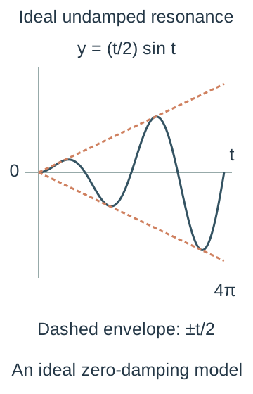
An undamped resonant example — For y″ + y = cos x, use y_PI = Cx sin x because the ordinary cosine/sine trial overlaps. Differentiating and substituting gives 2Ccos x, so y_PI = x sin x/2. The factor x produces an amplitude growing with the independent variable in this ideal undamped model.The particular response y=(t/2)sin t solves y″+y=cos t in the ideal undamped model. Dashed lines ±t/2 bound its growing oscillation envelope on 0≤t≤4π. The plot is not the bounded response of a positively damped oscillator and does not claim real physical motion can grow indefinitely without model limits.
Applying second-order conditions — For y″ + y = 0 with y(0) = 2,y′(0) = −3, the full family Acos x + Bsin x gives A = 2,B = −3. For forced equations include y_PI and its derivative before applying both conditions. Constants from two independent pieces cannot be chosen from only one condition without further information.
Verification before interpretation — Differentiate the proposed full solution twice and substitute into the original equation, then test initial conditions. Correct auxiliary roots do not guarantee a correct particular integral. Check signs, inner frequencies and any x factor introduced for overlap, as those errors often survive a superficial comparison of function shapes.
Kinematic models, harmonic motion and damping
State variables, signs and assumptions — A model needs an independent variable, dependent quantities, units and sign conventions before its differential equation is meaningful. Relate derivatives to the context: displacement derivative is velocity and its derivative is acceleration. Constant coefficients represent assumptions that may fail outside the observed range; mathematical exactness is not evidence that the physical assumptions are exact.
Motion with linear resistance — Take downward velocity v positive, gravity g > 0 and resistance proportional to velocity with coefficient leading to v′ + kv = g, k > 0. Then v = g/k + (v₀ − g/k)e⁻ᵏᵗ. The terminal velocity g/k balances gravity and resistance. The model assumes the linear drag law applies and does not represent every real-speed regime.
Displacement from a velocity model — Integrating that velocity gives s = s₀ + (g/k)t + ((v₀ − g/k)/k)(1 − e⁻ᵏᵗ). Check s(0) = s₀ and s′ = v. The coefficient k has reciprocal-time units after dividing the force equation by mass; a dimensional mismatch can reveal a missing mass or factor.
A cooling model — For constant ambient temperature T_a (the temperature of the surroundings), Newton-style cooling uses T′ = −k(T − T_a), k > 0. Its solution T = T_a + (T₀ − T_a)e⁻ᵏᵗ approaches the ambient temperature from either side. The model assumes a suitable proportional heat-transfer approximation and fixed ambient conditions; a changing ambient input requires a different equation.
The simple harmonic equation — Ideal displacement x(t) satisfying x″ = −ω²x with ω > 0 has solution x = Acosωt + Bsinωt. Acceleration is proportional to displacement and oppositely directed. Equilibrium is x = 0; constant positive acceleration is not simple harmonic motion.
Initial position and velocity in SHM — If x(0) = x₀ and x′(0) = u₀, then A = x₀,B = u₀/ω. The amplitude is R = √(x₀² + (u₀/ω)²) and period 2π/ω. For x₀ = 3,u₀ = 8,ω = 2, the motion is 3cos2t + 4sin2t, with amplitude five and period π.
Phase and speed relations — Write x = Rcos(ωt − δ) with Rcosδ = A and Rsinδ = B, choosing δ from both signs. Differentiating gives v² = ω²(R² − x²), so maximum speed is ωR at equilibrium. Squaring removes the sign of velocity; choose the correct sign from the actual direction of motion when needed.
Energy in ideal SHM — For unit mass, E = (1/2)v² + (1/2)ω²x² is constant because E′ = v(x″ + ω²x) = 0. With mass m and spring stiffness k, ω² = k/m and energy is mv²/2 + kx²/2. The ideal equation has no damping or external work, explaining rather than merely assuming constant amplitude.
The linear damped oscillator — With mass m > 0, damping c ≥ 0 and stiffness k > 0, free motion satisfies mx″ + cx′ + kx = 0. Its auxiliary equation is mr² + cr + k = 0. Resistance is proportional to velocity and opposes it. Translating a force law into this equation requires a consistent signed displacement from equilibrium.
Underdamped motion — If c² < 4mk and c > 0, x = e⁻ᶜᵗ⁄²ᵐ(Acosω_dt + Bsinω_dt), where ω_d = √(k/m − c²/(4m²)). The displacement oscillates within a decaying exponential envelope. The damped angular frequency is less than √(k/m); the latter is the undamped natural frequency.All curves solve x″+cx′+x=0 with x(0)=1,x′(0)=0 and the same mass/stiffness one. The solid c=1 response is underdamped; dashed c=2 is critical;(1+t)e⁻ᵗ; dotted c=3 is overdamped with two negative real rates. Common axes and initial data allow comparison; changing initial data can change monotonicity or crossings, so these plotted shapes do not describe every possible solution.
Critical damping — If c² = 4mk, the repeated-root solution is (A + Bt)e⁻ᶜᵗ⁄²ᵐ. There is no sinusoidal factor. Its shape still depends on initial conditions; it can pass through equilibrium without forming repeated oscillations. A repeated auxiliary root requires the linear factor t, which cannot be discarded because the envelope is decaying.
Overdamped motion — If c² > 4mk with c > 0, the roots are distinct negative real values and the solution is a sum of two decaying exponentials. It has no sustained sine/cosine oscillation. Different coefficients can produce a turning point or one crossing, so “nonoscillatory” does not mean every possible member is monotone for all times.
Damping and energy loss — For the unforced oscillator, E = mv²/2 + kx²/2 satisfies E′ = v(mx″ + kx) = −cv² ≤ 0. The energy decreases unless velocity is zero or damping vanishes. The result follows the assumed linear damping law and distinguishes the damped model from ideal constant-energy SHM.
Forced motion and transient response — A sinusoidal applied force gives mx″ + cx′ + kx = F₀cosΩt. The solution is a complementary transient (the part determined by initial conditions) plus a forced particular response. When c > 0 and m,k > 0, the complementary terms decay, leaving the bounded steady periodic response. With c = 0 a natural-frequency transient need not decay.
Steady response with nonzero damping — Try x_PI = AcosΩt + BsinΩt. Let D = (k − mΩ²)² + c²Ω². Then A = F₀(k − mΩ²)/D and B = F₀cΩ/D, where D ≠ 0. Its amplitude is F₀/√D for F₀ > 0. This follows from matching cosine and sine coefficients; damping produces a phase difference from the applied force.
Resonance and model limits — For c = 0 and Ω = √(k/m), D = 0 and the ordinary steady trial fails; a t-multiplied sinusoidal particular integral produces unbounded envelope growth in the ideal model. With positive damping, forcing at that same frequency has finite amplitude. The frequency of maximum damped displacement response need not equal the undamped natural frequency, so do not label every response peak by the same formula without deriving it.
Coupled first-order linear systems
Two dependent variables and one clock — A coupled linear model has X′ = aX + bY + f(t), Y′ = cX + dY + g(t), with constant coefficients and specified time inputs. Both unknowns depend on the same independent t. This compulsory form is linear in X and Y; a product XY is nonlinear and is not solved by the same elimination method without an additional approximation.
Eliminating one variable — When b ≠ 0, write Y = (X′ − aX − f)/b, differentiate the first equation and substitute Y′ and Y. This gives X″ − (a + d)X′ + (ad − bc)X = f′ − df + bg. Solve the resulting constant-coefficient second-order equation, then recover Y from the original first equation. If b = 0, solve the decoupled first equation or eliminate through another nonzero coupling.
A homogeneous coupled example — For X′ = X + 2Y and Y′ = 2X + Y, differentiation gives X″ − 2X′ − 3X = 0. Thus X = Ae³ᵗ + Be⁻ᵗ and Y = Ae³ᵗ − Be⁻ᵗ. The same constants occur in both expressions; independently adding two more constants to Y would overcount the two-dimensional solution family.
Initial data in both variables — For the previous system with X(0) = 3,Y(0) = 1, solve A + B = 3,A − B = 1 to get A = 2,B = 1. Hence X = 2e³ᵗ + e⁻ᵗ,Y = 2e³ᵗ − e⁻ᵗ. The initial value X′(0) = X(0) + 2Y(0) = 5 follows from the first equation and is not an independent arbitrary third condition.
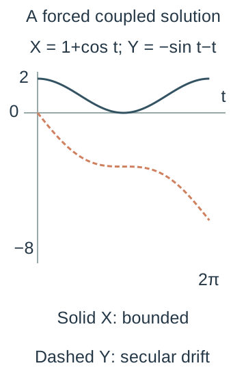
Coupled systems with time forcing — For X′ = Y + t and Y′ = −X, differentiate the first equation to get X″ + X = 1. Therefore X = Acos t + Bsin t + 1 and Y = X′ − t = −Asin t + Bcos t − t. Keeping the derivative of f(t) is essential; dropping it would incorrectly solve X″ + X = 0.
A forced coupled initial-value example — For that system with X(0) = 2,Y(0) = 0, A = 1,B = 0. Thus X = cos t + 1 and Y = −sin t − t. Verification gives X′ = −sin t = Y + t and Y′ = −cos t − 1 = −X. One variable is bounded while the other has a secular −t term, a nonoscillating part that grows in magnitude with time; inspect both before interpreting the model.The same solution pair X=1+cos t,Y=−sin t−t satisfies X′=Y+t,Y′=−X with X(0)=2,Y(0)=0. On the shared axes X remains between zero and two, while Y includes a downward secular −t term. Inspecting only X would miss the second state’s drift; whether either variable is physically meaningful depends on the stated context.
A linear interaction model and its limits — Linear coupled equations may approximate small deviations of two interacting populations, concentrations or linked quantities near a stated operating point. Coefficient signs encode the assumed effect of one on the other's rate. An unrestricted exponential or sinusoidal solution can become physically impossible for an absolute population, so interpret variables, time range and nonnegative constraints explicitly; do not claim to have solved a general nonlinear predator-prey system.
Verifying the full coupled solution — Substitute both functions and their derivatives into both original equations, including f(t),g(t), then test both initial values. A correctly solved eliminated equation can still be paired with a wrongly recovered Y. State the meaning, units and feasible range of each variable and distinguish mathematical instability from a proven real-world forecast.
Test yourself
50 questions · Random sets of 10. These quick checks support revision; practise longer explanations and justified judgements too.
 Mr Kidman's Classroom