Questions, data and measurement in geographical contexts
Start with the geographical claim — Choose information and methods to answer a question about location, pattern, process, scale or experience. A basin response question may need rainfall and discharge through time; a place-meaning enquiry may need situated accounts and representations. This chapter supports methods integrated across the course, not a replacement for applying them within water, carbon, global systems and actual place studies.
Primary and secondary describe the research relationship — Primary data are collected for the investigation, while secondary data were collected previously for another purpose or by another body. Both can be quantitative or qualitative and both require quality checks. A downloaded official dataset is not primary merely because the learner makes a new graph, and a personally conducted interview is not automatically unbiased.
Match data type to method — Counts, measured quantities, ranks, categories, text, images and audio support different analyses. Rainfall depth is a measured quantity; an agreed five-level environmental score is ordinal; an interview narrative can have multiple meanings that a simple score loses. Operational definitions state exactly how a concept is observed or measured: for example, which visible features earn each environmental score. State these definitions and preserve relevant detail rather than forcing every observation into a convenient numeric code.
Validity and reliability answer different questions — Validity concerns whether a measure addresses the intended concept; reliability concerns consistency under an appropriate repeat procedure. Repeatedly applying a narrow visual-quality score may be reliable without measuring every resident's well-being. Conversely, a relevant measure may be affected by inconsistent observers. Evaluate both the concept and the procedure in the actual context.
Precision does not guarantee accuracy — Precision concerns the fineness or repeatability of measurement, while accuracy concerns closeness to the relevant true value. A gauge reporting many decimal places can be systematically miscalibrated. Choose sensible resolution, check instruments and record uncertainty. Extra digits generated by a spreadsheet do not add information beyond the source measurements.
Random and systematic errors behave differently — Random variation may produce scatter among repeated readings; systematic error shifts results consistently through calibration, method or observer bias. More repeats can help estimate random variability but do not automatically remove a shared bias. For a channel measurement, an offset scale mark can affect every reading even if the readings agree closely.
Sampling needs a defined population and frame — Identify whether the population is people, locations, times or events, then specify the available sampling frame. A list excluding inaccessible streets or unregistered businesses can bias coverage before any selection is made. An event sample of one storm cannot represent every seasonal basin response. Match the target inference with the population actually covered.
Random, systematic and stratified designs have different uses — Random selection gives each included unit a known chance under its design; systematic selection uses a stated interval; stratification samples defined subgroups. Each needs a justified frame and implementation. A systematic interval can coincide with periodic land-use patterns, while stratification can improve subgroup coverage but needs a defined allocation. Convenience alone is not a probability design.
Space and time affect independence — Nearby sites, repeated readings from one location or several responses from one household may be related. Treating them as independent evidence can exaggerate the effective sample size. Design spatial and temporal coverage for the process, record repeated units and use appropriate analysis. More rows in a dataset do not necessarily mean more independent information.
Pilot, calibrate and document — A pilot can reveal unclear interview wording, unsafe access, impractical intervals or inconsistent scoring before full collection. Calibrate equipment where appropriate, define categories and record dates, locations, units, conditions and departures from the plan. A reproducible audit trail includes failed or missing observations with reasons rather than only the neat final table.
Cartography, spatial evidence and overlays
Use base, atlas and OS maps purposefully — A base map provides spatial reference, while atlas and detailed OS maps support different scales and questions. Read title, legend, orientation, scale, contour interval and date; identify which features are surveyed, symbolised or omitted. A national map of trade partners and a local catchment route map need different detail. Do not enlarge a small-scale map and assume it gains survey accuracy.
Convert scale before measuring distance or area — At 1:25,000, one centimetre represents 250 metres, so a straight practice distance of 4 cm represents 1 km. A curved route needs appropriate tracing rather than just endpoint separation. Area scales with the square of the linear conversion: one square centimetre represents 62,500 m² or 0.0625 km². State map projection and measurement limits where relevant.
Read coordinates and relief with context — Grid references or geographic coordinates locate observations within the chosen reference system; the datum (the reference model used for positions) and projection (how the curved Earth is represented on a flat map) matter when combining datasets. Contours join equal elevation and their spacing indicates slope under a stated interval. A close spacing suggests a steeper gradient than a wide spacing on the same map, not automatically a dangerous or inaccessible site under all conditions.
Field sketches and annotated photographs are analytical — Select features relevant to a process, mark viewpoint and direction, and separate observed form from inferred cause. A basin sketch can show channels, slopes and connected surfaces, while annotations explain possible pathways. A sketch is not required to reproduce every detail artistically; accuracy of relationships and transparent interpretation matter more than decorative shading.
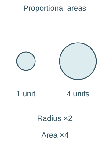
Located proportional symbols need the right scaling — Place symbols at the relevant nodes and size their areas in proportion to the measured quantity. If a circular symbol represents four times the quantity, its radius should double, not quadruple, because area is proportional to radius squared. Include a clear key, dates and units. Overlap and symbol placement can hide small but locally important values.The left circle represents one practice unit and the right four. The right radius is twice the left radius, making its area four times as large. These are illustrative symbols rather than mapped observations; quadrupling radius would wrongly multiply area by sixteen.
Flow, desire and trip lines answer different questions — A flow map represents movement with stated direction or magnitude. Desire lines connect origins and destinations directly to show demand or linkage, not necessarily the travelled route. Trip lines can depict actual journey paths under the defined mapping method. Label what the lines mean; a straight connection between two ports does not prove a ship followed that exact path.
Choropleth maps require comparable area indicators — Shade defined areas using suitable rates, proportions or densities, with a legend and justified class intervals. Raw population totals can be dominated by area size or boundary design and need particular caution. Within-area variation is hidden, and colour can exaggerate differences around a class boundary. An area category does not identify every individual's characteristics.
Isolines interpolate a continuous field — An isoline joins equal values such as rainfall depth or elevation. Its location depends on sampled points, spacing and interpolation assumptions, and it may be uncertain where observations are sparse. A smooth rainfall surface is not a direct measurement at every pixel. Use plausible continuity and show underlying data or uncertainty where useful.
Dot maps need a clear meaning — In a dot-density map, each dot may represent a stated number of people or events placed within an area under a mapping rule; it need not mark exact addresses. In a point map, a dot may instead locate an actual observation. The legend must distinguish these. Avoid exposing sensitive locations or reading an allocated density dot as a particular household.
Overlays and weather maps need compatible layers — Physical transparencies or GIS layers can compare land use, slope, access and observations, but align scales, dates, coordinates and classifications first. Where synoptic charts are relevant to a rainfall event, read pressure, fronts, wind and timing from the legend and evidence; a pressure pattern alone does not establish the measured local rainfall total. Record which layers are observations and which are modelled.
Graphs and visual comparison in context
Choose the display for the variable and question — A hydrograph needs time and discharge, a trade composition comparison needs categories or shares, and an interview analysis needs contextualised themes as well as any counts. Include an informative title, units, sample basis, dates and source. Select a graph because it reveals a relevant pattern, not because software offers a visually impressive default.
Simple and comparative lines show ordered change — A line can connect successive time measurements such as discharge; comparative lines show several compatible series on a clear shared scale. Connecting unordered categories can imply continuity that is not meaningful. Gaps should remain visible where data are missing rather than being silently filled. Different sampling intervals must be represented accurately along the time axis.
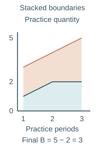
Compound lines require care with stacked values — A compound or stacked line display can show components accumulating to a total, such as sources within a compatible water account. The upper line is a cumulative boundary, not necessarily the value of the last component alone. Read each component as the vertical difference between relevant boundaries. Stacking unrelated units or double-counted transfers creates a misleading total.Invented components A and B across three practice periods are A=(1,2,2) and B=(2,2,3). The lower blue boundary shows A; the orange upper boundary shows A+B=(3,4,5). At the final period, B is the vertical difference 5−2=3 rather than the upper cumulative value five. The axis uses equal numerical spacing.
Bars compare categories and can be grouped or stacked — Simple bars compare categories, comparative bars place matched groups side by side, and compound bars divide a total into components. Equal-width bars and a meaningful baseline support fair comparison. A percentage stack compares composition but can conceal different absolute totals. State whether the display uses counts, rates or percentages and whether parts genuinely sum to the whole.
Divergent displays need a meaningful reference — Bars or lines extending on opposite sides of zero can show positive and negative change, a balance or deviation from a baseline. The sign must have a defined meaning: a negative storage change is a loss, not a negative amount of water existing. Use compatible reference periods and avoid comparing deviations from different baselines as if identical.
Scatter graphs explore paired relationships — Plot two measurements for the same unit, such as practice site rainfall and runoff, with labelled axes and appropriate ranges. Describe direction, form, strength, clusters and unusual points before calculating a coefficient. A line of best fit summarises a modelled trend and need not pass through the origin; it is not formed by joining every point in sequence.
Best-fit lines have a scope — A fitted relationship can support interpolation within observed conditions if its assumptions are plausible. Extrapolation beyond the observed range or to another basin may fail. Outliers can reflect error or genuine process differences and should be investigated rather than deleted solely to improve fit. A good fit does not establish which variable causes the other.
Pie charts and divided circles encode parts and totals — Angles in a pie chart represent shares of a whole that sum to 100%; an invented 25% category occupies 90°. Proportional divided circles can show composition and differing totals, with circle area scaled to the total. A radius proportional to the total would exaggerate area differences. Too many thin sectors can prevent useful comparison.
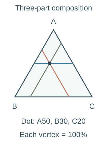
Triangular graphs represent three-part composition — A triangular graph plots three non-negative components that sum to a fixed total, usually 100%. Each vertex represents 100% of one component, with values read using the chart's specified axis directions and parallel grid lines. An invented composition of 50%, 30% and 20% is valid; 50%, 40% and 30% cannot be plotted as one percentage composition without correcting the account.The dot represents invented shares A=50%, B=30% and C=20%. A is read on the horizontal blue line parallel to BC; B on the orange line parallel to AC; C on the green line parallel to AB. Each vertex is 100% of its labelled component. The lines intersect at the same composition, whose shares sum to 100%.
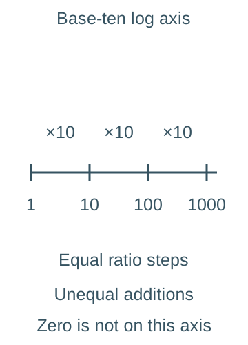
Logarithmic scales show ratios rather than equal differences — On a base-ten logarithmic axis, 1, 10, 100 and 1000 are equally spaced. They represent equal multiplicative steps, not equal additions; zero and negative values cannot be placed on that ordinary log scale. Such a display can compare widely differing trade volumes, but readers must know the scale and must not infer linear absolute change from equal vertical gaps.The labelled base-ten axis places 1,10,100 and 1000 at equal intervals, each a tenfold step. The absolute increases are nine, ninety and nine hundred, so equal visual gaps are not equal additions. Zero and negative values cannot be placed on this ordinary logarithmic axis.
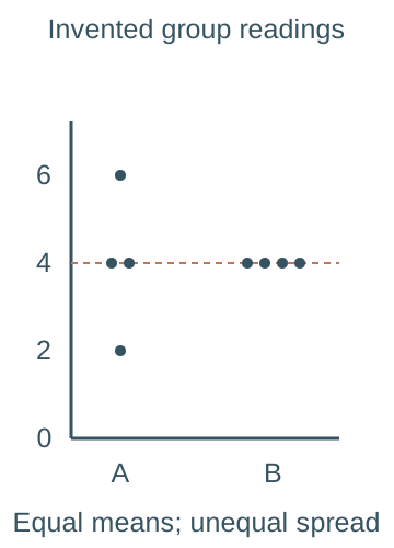
Dispersion diagrams retain individual variation — Plot individual values for each group along a common numerical scale, arranging overlap clearly and recording sample sizes. They can reveal spread, clusters and outliers hidden by a mean, such as differing practice infiltration readings. Do not spread horizontal positions as if they measure another variable unless they do; label any jitter as a display aid.The invented group A readings are 2,4,4,6 and group B readings are 4,4,4,4, with n=4 in each. Both means equal four, shown by the dashed horizontal level, while A is more dispersed. Small horizontal offsets separate overlapping points and are display jitter, not another measured variable.
Descriptive statistics and their limits
Central tendency needs an appropriate measure — The mean adds values and divides by their count; the median is the middle ordered value or mean of the two middle values; the mode is the most frequent value or category. An extreme reading can strongly affect a mean while leaving the median less changed. State the unit and distribution, and do not compute a meaningful numerical mean of arbitrary category codes.
A worked descriptive account — For invented readings 2, 4, 4 and 6, the mean is 4, median is 4 and mode is 4. The range is 6 − 2 = 4. Using medians of the lower and upper halves gives Q1 = 3 and Q3 = 5, so IQR = 2. This is an explicit quartile convention; software methods can differ for small samples.
Range and interquartile range reveal different spread — Range uses the extreme values and is sensitive to unusual readings. IQR describes the span of the middle half under the stated quartile convention and is less affected by extremes. Neither alone describes the full shape. Two groups can have the same median but different variability, which matters for reliability or unequal place experiences.
Standard deviation uses deviations from the mean — A descriptive population standard deviation is √[Σ(x − x̄)²/n] for the complete defined set. Here Σ means add all the terms, x is each value, x̄ is the mean and n is the number of values. For 2, 4, 4 and 6, squared deviations sum to 8, giving variance 2 and standard deviation √2, approximately 1.414. Squaring avoids cancellation of positive and negative deviations; the final square root restores the original measurement unit.
Sample and population calculations differ — When using a sample to estimate population variance, a common formula divides the squared-deviation sum by n − 1 rather than n. For the same four readings this gives sample variance 8/3 and sample standard deviation about 1.633. State which formula the question or analysis requires and keep it consistent rather than mixing outputs from different software defaults.
Difference and association are distinct claims — A difference compares groups or periods, such as average readings in two surfaces. Association asks whether paired variables vary together, such as their ranks across sites. Descriptive patterns can suggest a process but are not automatically statistically significant or causal. Choose a method for the actual question rather than applying a familiar test to every table.
Uncertainty includes more than a summary statistic — A small standard deviation within a biased sample does not guarantee the estimated area mean is accurate. Sampling design, spatial dependence, calibration, missing values and operational definitions affect confidence. Report the statistic alongside sample size, coverage and limitations. Do not hide inconvenient variability by presenting only a rounded mean.
Spearman, Chi-square and significance in context
Inference requires a defined hypothesis and design — Inferential procedures compare observed evidence with a stated null model under assumptions. A null hypothesis usually proposes no association or no difference; the alternative describes the association or difference being tested. Specify the population, sampling process, variables, significance level and appropriate alternative before interpreting a result. A test cannot repair biased recruitment or turn repeated dependent observations into independent evidence. Practice calculations here are invented and are not a learner's field results.
Spearman assesses monotonic rank association — Spearman's coefficient describes how consistently paired ranks rise or fall together. Use paired observations of two rankable variables for the same sampling units and consider whether a monotonic relationship is sensible: as one variable increases, the other generally moves in one direction, even if the rate changes. A coefficient near +1 or −1 indicates strong rank agreement or reversal; near zero need not mean no possible nonlinear relationship. Correlation alone does not establish causation.
Rank both variables consistently — Order each variable using the same ascending or descending convention, keeping each original pair together. Equal values receive the mean of the ranks they occupy. For values 10, 10 and 20, ascending ranks are 1.5, 1.5 and 3. Ties reduce distinct ordering information and require the appropriate coefficient and significance procedure.
The untied shortcut has a condition — With no tied ranks, rₛ = 1 − 6Σd²/[n(n² − 1)], where d is each pair's rank difference. With ties, compute the Pearson correlation of the average-rank columns or use an appropriate tie-aware method; do not assume that inserting average ranks into the untied shortcut gives the exact same coefficient. Record the method used.
A worked rank coefficient — For paired rank columns X = (1,2,3,4,5) and Y = (1,3,2,5,4), differences are (0,−1,1,−1,1) and Σd² = 4. With n = 5, rₛ = 1 − 24/120 = 0.8. This describes a positive rank association within a very small invented sample; it does not by itself establish a significant population relationship.
Use the appropriate significance comparison — Compare the absolute coefficient with a suitable two-sided critical value for the sample size and method, or use an appropriate p-value. A p-value is the probability, assuming the null model and its conditions, of a result at least as extreme as the one observed; it is not the probability that the null hypothesis is true. If the task supplies a 5% two-sided critical magnitude of 1.00 for the preceding untied n = 5 case, 0.8 does not reach it. A one-sided test, ties or a different sample size changes the relevant procedure; do not use an unrelated table.
Chi-square independence uses categorical counts — A Pearson Chi-square test of independence compares observed cell counts with expectations under no association between two classifications. Observations must be appropriately sampled and independent, with each counted once in mutually exclusive cells. Use frequencies rather than percentages or continuous raw measurements, and check expected counts are sufficiently large for the approximation.
Construct expected counts from the margins — For an independence table, E = row total × column total / grand total for each cell. An invented two-place yes/no table has rows (30,20) and (10,40), giving row totals 50 and 50, column totals 40 and 60, and total 100. Both rows therefore have expected counts (20,30), not equal expectations of 25 in every cell.
Calculate and compare the Chi-square statistic — O means an observed count and E its expected count under independence. For that invented table, χ² = Σ(O − E)²/E = 100/20 + 100/30 + 100/20 + 100/30 = 50/3, about 16.67. With two rows and two columns, df = (2 − 1)(2 − 1) = 1. The uncorrected Pearson statistic exceeds a supplied upper-tail 5% critical value of about 3.84, so reject independence if the design assumptions hold.
Check sparse cells and the test variant — A conservative teaching check is that all expected counts are at least five; sparse tables may need a justified exact method or appropriate category combination rather than blind use of the approximation. Do not combine categories merely to obtain a preferred result. A continuity-corrected 2×2 calculation is a different procedure from the explicitly uncorrected example, and a goodness-of-fit test has a different hypothesis and degrees-of-freedom account.
Interpret significance without claiming proof — At a 5% threshold, a significant result is evidence against the null under the model and design, not a 95% probability that a preferred causal explanation is true. Failing to reject does not prove no relationship; small samples may have limited power. Statistical significance, effect size, geographical importance, uncertainty and causal mechanism are separate questions.
Digital, qualitative and ethical evidence across themes
GIS links spatial data with attributes — A geographical information system (GIS) can store, query, overlay and display location-referenced information such as basin land cover, transport connections or place-study indicators. Coordinate reference systems, resolution and time must be compatible. A visually persuasive overlay does not prove causation; investigate process, uncertainty and the spatial unit used for analysis.
Remote sensing needs interpretation and validation — Satellite or airborne sensors record radiation or other signals that can be interpreted as land cover, surface conditions or change. Cloud, season, sensor resolution and classification error affect comparisons. Ground checks and metadata help assess meaning. A classified map is an analytical product, not a direct observation of every social or ecological property assigned to a colour.
Electronic databases need an audit trail — Record dataset version, extraction date, definitions, filters, missing-value codes and transformations. Preserve raw data and calculate in a separate reproducible process. A blank may mean not collected rather than zero. Check spreadsheet formulas, sorting and paired rows, because an accidental column shift can create a false correlation without changing any individual number.
Crowd sourcing can widen coverage unevenly — Publicly contributed sightings, photographs or reports may provide rich spatial and temporal detail. Participation depends on connectivity, interest, access and reporting behaviour, so many contributions do not guarantee representative coverage. Validate location and duplication, distinguish absence of a report from absence of the phenomenon and protect contributor privacy.
Big data does not automatically remove bias — Large volumes of transactions, movement records or platform activity can reveal patterns but reflect who uses the system, what is recorded and how algorithms filter it. Device or account counts are not automatically people, and proprietary methods can limit transparency. More records can increase precision around a biased estimate rather than making it accurate.
Qualitative methods actively construct accounts — Interview questions, setting, recruitment, transcription, coding and presentation influence the representation produced. Define themes transparently, retain contrary accounts and reflect on researcher position. Coding counts describe the analysed material, not automatically the wider population. Use contextual explanation alongside numerical summaries when investigating meanings and mechanisms.
Ethics applies to maps numbers and narratives — Explain informed participation, confidentiality, data minimisation, storage and appropriate use. Combining public datasets or geolocated accounts can re-identify individuals or expose sensitive communities even if each source seems harmless alone. Consider who benefits, who may be harmed and whose categories or interpretations dominate. Follow the school's actual procedures rather than inventing consent for real participants.
Communicate a geographical argument — Present a sequence from question and theory through methods, located evidence, analysis and evaluated conclusion. Use labelled maps, graphs, quotations and statistics where they support specific claims, and discuss misuse, uncertainty and alternatives. A polished export or a significant test does not replace explanation of the geographical process and the limits of the evidence.
Test yourself
50 questions · Random sets of 10. These quick checks support revision; practise longer explanations and justified judgements too.
 Mr Kidman's Classroom