Positive exponential base — For a > 0, the function y = aˣ is defined for every real x and has positive output. When a > 1 it increases, while 0 < a < 1 gives a decreasing graph. The case a = 1 is the constant function one and does not have a logarithmic inverse on all real inputs.
Intercept and asymptote — For a positive base different from one, a⁰ = 1 so the graph passes through (0,1). The horizontal axis y = 0 is an asymptote in the direction where the outputs decay toward zero. No finite real input produces a zero output for the pure exponential aˣ.
Base e — The constant e is approximately 2.71828 and is the base of the natural exponential. The graph y = eˣ has the distinctive property that its gradient equals its output at every input. This is an exact structural property, not a claim that every exponential aˣ has gradient aˣ.
Scaled exponential gradient — For y = eᵏˣ, dy/dx = keᵏˣ. The notation dy/dx means the instantaneous rate at which y changes as x changes, also called the derivative or graph gradient. Thus the rate of change is proportional to the current value with constant k. If k > 0 the output increases, if k < 0 it decreases, and k = 0 gives constant one. Later differentiation methods justify the chain-rule calculation more generally.
Amplitude multiplier — For y = Aeᵏˣ with constant A, the derivative is kAeᵏˣ = ky. A is the initial value y(0); its sign determines whether the graph lies above or below zero. In a nonnegative population or mass model, a negative initial A would be physically inadmissible even though algebraically defined.
Translated exponential — The graph y = e2x − 1 + 3 has horizontal asymptote y = 3, domain all real x and range y > 3. Its y-intercept is 3 + e⁻¹. The exponent's horizontal shift can be read by writing 2(x − 1/2); the outer addition moves the limiting level.
Shifted rate relationship — If y = L + Aeᵏˣ, then dy/dx = k(y − L), not ky unless L = 0. The rate is proportional to deviation from the limiting level. A fictional temperature-like curve 20 + 80e−0.2t starts at 100 and approaches 20; the exponential part tends to zero while the whole output does not.
Magnitude and direction — An exponential curve with A > 0 and k < 0 approaches its baseline from above, while A < 0 with the same negative k approaches it from below. Interpret the sign of the derivative and the offset together. Decreasing exponential factor alone does not mean every translated/scaled output decreases.
Rates and units — In eᵏᵗ the exponent must be dimensionless, so k has reciprocal-time units, such as s⁻¹ meaning per second, when t is time. Changing from days to hours changes k's numerical value. Keep the same time unit in both calibration and prediction, and distinguish a rate constant from a percentage increase over one finite period.
Logarithmic inverses graphs and laws
Logarithm definition — For a > 0, a ≠ 1 and x > 0, logₐx is the exponent y satisfying aʸ = x. Thus log₂8 = 3 because 2³ = 8. A real logarithm does not accept zero or negative arguments; logₐ0 is undefined, not zero.
Natural logarithm — The function ln x means log base e and is the inverse of eˣ. Its domain is x > 0, range is every real number, and ln 1 = 0. Conversely e⁰ = 1 and ln e = 1. The logarithm's output can be negative even though its input must be positive.
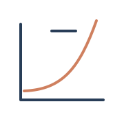
Logarithm graph — For a > 1, logₐx increases, passes through (1,0) and has vertical asymptote x = 0. For 0 < a < 1 it decreases instead. The graph is the reflection of the corresponding exponential in y = x, exchanging domain and range.The green eˣ and brown ln x graphs use equal scales of 60 pixels per input/output unit and reflect in the dashed line y=x. Dark points mark (0,1) and (1,0). The plotted viewport shows finite curve segments; ln x continues toward its vertical asymptote at x=0 and eˣ approaches y=0 in the other direction.
Inverse identities — Ln(eˣ) = x for every real x, while eln x = x requires x > 0. Similarly logₐ(aˣ) = x on real inputs and alogₐ x = x on positive inputs. Record which expression contains a logarithm before cancelling inverse symbols.
Product law — For x > 0 and y > 0, logₐx + logₐy = logₐ(xy). For example ln 2 + ln 5 = ln 10. The inputs need separate positivity; a positive product of two negative numbers does not make their individual real logarithms defined.
Quotient law — For x,y > 0, logₐx − logₐy = logₐ(x/y). In particular ln 12 − ln 3 = ln 4. Subtraction inside a logarithm does not follow the same rule: ln(x − y) is not generally ln x − ln y.
Power law — For x > 0 and real k, k logₐx = logₐ(xᵏ). Hence ln(1/x) = −ln x and ln√x = (ln x)/2 on positive inputs. The exponent moves out as a multiplier; it does not multiply the logarithm's argument instead.
Squares and negative inputs — Ln(x²) is defined when x ≠ 0 and equals twice ln of the magnitude of x. The expression 2 ln x is defined only for x > 0. Replacing ln(x²) by 2 ln x without preserving a negative-input possibility can wrongly remove valid inputs from a larger problem.
No addition law — There is no general law ln(x + y) = ln x + ln y. With x = y = 1, the first side is ln 2 while the second is zero. Keep an un-factorised sum intact, or use justified algebra before applying a product law.
Change of base — For x > 0 and valid positive bases a,b different from one, logₐx = log_bx/log_ba. Thus log₂3 = ln 3/ln 2. The denominator is nonzero because a ≠ 1, and a calculator's natural or base-ten logs can evaluate an otherwise unavailable base.
Exact logarithmic answers — Expressions such as ln 3/ln 2 are exact values, whereas a decimal approximation should use ≈ and requested precision. Retain full intermediate precision when the logarithm is later used to decide an integer threshold. Early rounding can change which step is first admissible.
Exponential and logarithmic equations and inequalities
Matching powers — If a > 0 and a ≠ 1, the exponential is one-to-one, so aᶠ⁽ˣ⁾ = aᵍ⁽ˣ⁾ implies f(x) = g(x). For 3ˣ = 27 = 3³, x = 3. Do not use one-to-one reasoning with base one, where every exponent gives the same output.
Taking logs of powers — To solve aˣ = b with a,b > 0 and a ≠ 1, take logs to get x = ln b/ln a. For 23x − 1 = 3, (3x − 1)ln 2 = ln 3, giving x = (1 + ln 3/ln 2)/3. The input exponent is the whole expression 3x − 1.
Natural-exponential equation — For e2x + 1 = 7, take ln to obtain 2x + 1 = ln 7 and x = (ln 7 − 1)/2. A negative right-hand target for the pure exponential would instead give no real solution. A shifted exponential target must be isolated before deciding positivity.
Logarithmic equation — For ln(2x − 1) = 3, the domain requires x > 1/2. Exponentiate to obtain 2x − 1 = e³, so x = (e³ + 1)/2, which satisfies the restriction. The operation reverses the logarithm; it does not mean multiply both sides by e.
Equal logarithms — If two real logarithms have the same valid base, equality of their arguments follows. For ln(x + 2) = ln(3x), require x > 0, then solve x + 2 = 3x to get x = 1. Check argument positivity rather than assume every root of the rearranged equation is valid.
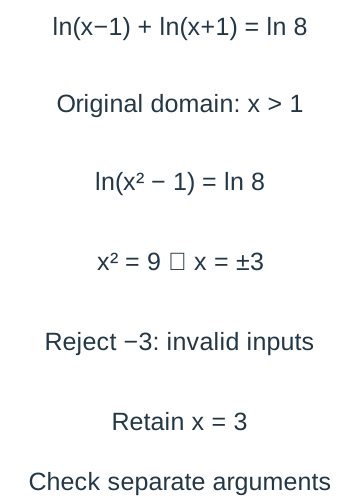
Combining logarithms with domains — For ln(x − 1) + ln(x + 1) = ln 8, the original domain is x > 1. Combining gives ln(x² − 1) = ln 8, so x² = 9 and x = ±3. Only x = 3 lies in the original domain; a positive combined product alone would wrongly admit −3.Each original logarithm requires a positive argument, giving x>1 before any product-law combination. The algebraic equation x²=9 supplies two candidates, but x=−3 makes both original individual arguments negative. Only x=3 is valid; the positive combined product at −3 cannot repair the undefined original logarithms.
Exponential quadratic — For 4ˣ − 5·2ˣ + 4 = 0, use u = 2ˣ > 0 and solve u² − 5u + 4 = 0. Then u = 1 or 4 gives x = 0 or 2. A negative auxiliary root in a different exponential quadratic would be rejected because real 2ˣ is always positive.
Increasing-base inequality — For 2ˣ > 8, the increasing exponential gives x > 3. More generally, after isolating a positive exponential target, taking an increasing logarithm preserves direction, but dividing by ln a requires checking its sign. State the domain and base conditions before applying a memorised comparison.
Decreasing-base inequality — For (0.8)ⁿ < 0.1, taking ln gives n ln 0.8 < ln 0.1. Since ln 0.8 is negative, n > ln 0.1/ln 0.8, approximately 10.32. If n counts whole steps, the first allowed integer is 11; check n = 10 and 11 in the original condition.
Original-equation verification — Substitute a proposed answer into the original equation with every denominator, logarithm and physical restriction intact. Exponentiating or combining logarithms may produce an equation with a broader apparent domain. Keep exact working until the final approximate output and explain why any rejected branch fails.
Logarithmic plots and parameter estimation
Power-law linearisation — For y = axⁿ with a,x,y > 0, linearisation means transforming variables so the model becomes a straight-line relationship. Taking natural logs gives ln y = ln a + n ln x. Plot ln y vertically against ln x horizontally to obtain a straight line of gradient n and intercept ln a when the model holds. The exponent is the gradient, while the original coefficient is obtained by exponentiating the intercept.
Base-ten power plot — Using base-ten logs gives log₁₀y = log₁₀a + n log₁₀x. A line with gradient 3/2 and vertical intercept 2 represents y = 100x³ᐟ², not y = 2x³ᐟ². The logarithm base determines how the intercept is converted back; the power-law exponent is unchanged.
Power model from two points — If y = axⁿ passes through positive data (1,3) and (4,24), then a = 3 and 4ⁿ = 8, so n = 3/2. The model is y = 3x³ᐟ². These two points determine the parameters but do not prove that the same relationship fits all other observations.
Exponential linearisation — For y = kbˣ with k,b > 0, ln y = ln k + x ln b. Plot ln y against x, giving gradient ln b and intercept ln k. This is a different horizontal variable from the power-law log-log plot; label the axes fully so the inferred parameters are meaningful.The two transformations have different horizontal variables. A power law produces slope n on a log-log plot, while an exponential produces slope ln b on a log-output versus original-input plot. Both intercepts are logged original coefficients and must be exponentiated in the chosen base to recover those coefficients.
Natural rate form — For y = Aeᵏˣ with A > 0, the same plot has equation ln y = ln A + kx. Its slope is k directly, while A is e raised to the intercept. If base-ten logarithms are plotted instead, the slope is k/ln 10; using the wrong base changes the estimated rate.
Exponential data example — A model y = kbˣ through (0,5) and (2,20) has k = 5 and b² = 4. With the exponential base required positive, b = 2, giving y = 5·2ˣ. The ln plot's intercept is ln 5 and slope ln 2; do not retain b = −2 as an all-real-input exponential model.
Reading transformed slopes — A base-ten plot of log y against x with slope 0.02 gives b = 100.02 in y = kbˣ. A log-log plot with the same slope instead gives power exponent n = 0.02. The number alone is insufficient without the plotted variables, units and log base.
Choosing and testing a model — A roughly straight log-log graph suggests a power law; a roughly straight log-y versus x graph suggests an exponential. Examine additional data, deviations and context before concluding a model is appropriate. Two points always lie on a line in a transformed plot and cannot test the pattern's wider consistency.
Plotting restrictions and units — Real logarithmic plots require positive plotted quantities. A zero or negative observation cannot be silently omitted or changed to one merely to obtain a straight line. Use numerical measurements in stated consistent reference units; changing those units can alter the intercept and coefficient, so report the original quantities and units with the fitted equation.
Growth decay limiting behaviour and model evaluation
Continuous growth model — A fictional population N(t) = 200e0.03t has initial value 200 at t = 0 and instantaneous proportional rate 0.03 per chosen time unit. Its output is positive and increases without bound in the mathematical model. State the time unit and explain why indefinite resource-free growth is a simplification.
Discrete versus continuous rates — A finite-period multiplier of 1.04 corresponds to continuous rate k = ln 1.04, approximately 0.03922 per period, because eᵏ = 1.04. Conversely continuous k = 0.04 gives finite-period increase e0.04 − 1, approximately 4.081%, not exactly 4%. Keep the distinction explicit when translating a percentage statement into a model.
Growth calibration — For N = Aeᵏᵗ, an observation at t = 0 gives A directly. Given positive observations N₁,N₂ at distinct times t₁,t₂, divide to obtain k = ln(N₂/N₁)/(t₂ − t₁). Use the same time unit and check whether the data support a constant proportional rate rather than assume it from two observations.
Doubling time — With positive growth rate k, doubling requires eᵏᵀ = 2, so T = ln 2/k. At k = 0.04 per year the doubling time is approximately 17.33 years. It is independent of the initial positive amount within this fixed-rate model, but changes if the proportional rate changes.
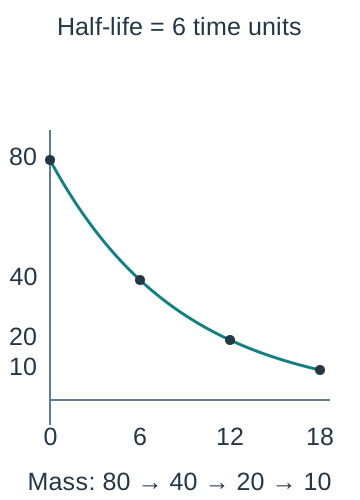
Decay and half-life — For M(t) = M₀e⁻ᵏᵗ with k > 0, the half-life T satisfies e⁻ᵏᵀ = 1/2, giving T = ln 2/k. A fictional material of initial mass 80 and half-life 6 time units has M(t) = 80e−(ln 2)t/6; after 18 units three halvings leave mass 10. These are mathematical illustrations rather than measurements of a named substance.The fictional mass model has initial mass 80 and half-life six time units. Dark points at t=0,6,12,18 have masses 80,40,20,10. The horizontal axis uses 15 pixels per time unit and the vertical axis 3 pixels per mass unit. Equal horizontal intervals halve the remaining amount rather than remove the same fixed mass each time.
Threshold times — For the fictional population to reach 500, solve 200e0.03t = 500, giving t = ln(5/2)/0.03, approximately 30.54 time units. If the question asks for the first whole census time with at least 500, test the surrounding integers and choose 31. Continuous event time and first discrete observation are different answers to different questions.
Nonzero limiting level — The model y(t) = 20 + 80e−0.2t approaches 20 as t grows and has y(0) = 100. Solving for a target first requires subtracting 20; targets below or equal to the asymptotic level are not reached at finite nonnegative time in this model. Its rate is −0.2(y − 20), consistent with approach from above.The curve y=20+80exp(−0.2t) begins at 100 when t=0 and stays above the dashed baseline y=20 at every finite nonnegative t. Horizontal scale is 20 pixels per time unit and vertical scale 2.5 pixels per output unit. The output rate is proportional to deviation from 20, not the entire output.
Physical domain and output — A population model may be used only for t ≥ 0 or a stated observation range, even though its algebra accepts negative t. Counts are intrinsically discrete, so a continuous output may be an estimate requiring interpretation rather than an exact fractional person. A positive exponential does not by itself establish that every output is plausible.
Refining a model — Resource limits can make a bounded population model more plausible than unlimited exponential growth. A nonzero background level can justify an offset exponential in a decay context. Identify the actual mismatch, state any extra parameters or assumptions and compare further observations; adding complexity without evidence does not guarantee a better prediction.
Uncertainty and extrapolation — Small changes in an estimated rate can produce large differences over long extrapolations. Report approximate parameters with appropriate precision, inspect fit over the observed interval and qualify future predictions by the model's assumptions. The fictional rates and balances used in these chapters are teaching examples, not current financial products or forecasts.
Test yourself
50 questions · Random sets of 10. These quick checks support revision; practise longer explanations and justified judgements too.
 Mr Kidman's Classroom