K5MA17 · Forces, Newton's laws, friction and connected particles · Edexcel A-level Mathematics

Revise the key ideas

Forces free-body diagrams and modelling assumptions

Force as an interaction — A force is a directed interaction acting on a specified body. Identify which body a diagram describes and which external objects exert its forces. Force magnitude alone does not determine its effect on acceleration; direction and the combined resultant matter.
Mass and weight — Mass measures inertia, resistance to a change in velocity under a given force, and is measured in kilograms; weight is the gravitational force mg in newtons. In a near-surface model g is usually 9.8 m/s² unless another value is supplied. A 5 kg body has weight 49 N under that assumption, not mass 49 kg; g and weight can vary with location while mass remains the same.
Normal reaction — A normal contact force acts perpendicular to the contacting surface. On a horizontal surface it is vertical, but on an incline it is not. Its magnitude is determined by the force balance or normal acceleration, not automatically equal to mg. A simple nonadhesive contact can push but cannot pull the body towards the surface.
Tension — A taut light string pulls a body along the string away from its point of attachment. A string does not push. A negative calculated tension signals that the assumed taut-string stage or geometry is inconsistent, rather than a physical compressive string force.
Thrust compression and resistance — A rod or supporting contact may push through compression or pull depending on its construction; a string cannot support compression. Resistance is a force opposing relative motion in its stated model. Do not automatically assign every resistance the same direction as negative acceleration; actual motion and interaction determine its direction.
Free-body diagram — Draw only forces acting on the chosen body, with labels and directions: weight, contacts, tensions, friction and applied forces as appropriate. Do not add velocity or ma as extra physical forces. Acceleration can be marked separately as a kinematic direction to organise the equations.
Choosing coordinate axes — Choose perpendicular axes convenient for the motion or constraints, often along and normal to a slope. Resolve every force into those same axes and assign signs consistently. An angled force can contribute to both equations; a surface being horizontal does not imply every applied force is horizontal.
Particle model — Treating a body as a particle neglects its size and rotation, allowing translational force equations at a point. It cannot on its own answer whether a long object tips or rotates; moments and rigid-body geometry are needed for those questions. State which model is being used rather than combine incompatible assumptions silently.
Light and inextensible strings — A light string has negligible mass in the ideal model; inextensibility fixes its length while taut. For a simple two-body connected arrangement, the latter links their acceleration magnitudes along the string. The bodies may accelerate in different spatial directions, and slack or stretch changes the constraint.
Smooth and rough contacts — Smooth means friction is neglected at that contact. A rough contact may support a tangential friction force following a specified model. Smooth does not mean weight, normal force or acceleration is zero; state exactly which interaction has been omitted.

Newton's laws resultants and components

First law and inertial frame — An inertial frame is a nonaccelerating reference frame in which Newton's first law applies. In such a frame, zero resultant force gives constant velocity, which can include rest. A moving particle does not require a forward resultant merely to continue at constant velocity. A forward driving force may be balancing resistance so the net force is zero.
Second law — For a constant-mass particle in an inertial frame, ΣF=ma, with vector or component equality. ΣF is the resultant of all included external forces acting on that particle. The unit newton is kg m/s²; mass times acceleration is the consequence of the resultant, not an additional force to draw.
Component equations — Resolve ΣFₓ=maₓ and ΣFᵧ=maᵧ along chosen perpendicular axes. A zero acceleration component gives a zero resultant component on that axis, even if acceleration along the other axis is nonzero. Check which motion constraints justify setting any component to zero.
Worked vector resultant — For a 2 kg particle with external forces (6,1) N and (−2,5) N, the resultant is (4,6) N and acceleration (2,3) m/s². Acceleration magnitude is √13 m/s². Divide each resultant component by mass before interpreting direction or magnitude.
Third law — When body A exerts a force on body B, B exerts an equal-magnitude opposite force on A of the same interaction type. The pair acts on different bodies, so it does not cancel within a free-body diagram for one body. The two forces occur together rather than as a delayed response.
The schematic illustrates a repulsive interaction between bodies A and B. The leftward force belongs on A and the equal rightward force on B. Arrow lengths are equal to express the third-law equality; forces on different bodies are not combined into one single-body balance. Other external interactions are not asserted absent by this interaction-pair illustration.
Weight and support are not a third-law pair — A stationary body's weight and normal support can balance but are both forces on that body. The partner of its weight is its gravitational force on Earth; the partner of the support is its force on the supporting surface. Equal opposite directions alone do not identify a third-law interaction pair.
Equilibrium of a particle — For a particle in equilibrium, the resultant is zero, so both perpendicular component sums vanish. This can describe rest or constant translational velocity in the inertial model. Particle force equilibrium alone does not prove rotational equilibrium for a finite rigid body.
Resolving an angled force — A force P at angle θ above a horizontal positive axis has horizontal component Pcosθ and upward component Psinθ. An angle measured from a vertical or slope-normal axis changes the component assignments. Draw the right triangle and use the actual stated reference angle.
Force triangle — For three coplanar forces, forces acting in the same plane, in particle equilibrium, a head-to-tail vector construction closes. It can support sine/cosine rule calculations when the labelled directions are known. A triangle drawn with arbitrary angles does not replace resolving the actual forces or checking which physical forces act.
Unknown forces and consistency — Use sufficient independent component equations for the unknown force magnitudes and directions, then test sign and contact constraints. A numerical answer with a negative normal reaction or tension may indicate loss of contact or slack, requiring a different stage model. Do not turn it positive by taking an absolute value without interpreting the changed physics.

Horizontal surfaces vertical motion and contact constraints

Smooth horizontal acceleration — For a body on a smooth horizontal plane with only horizontal applied force P and weight/support vertically, zero vertical acceleration gives R=mg while horizontal acceleration is P/m. R=mg here follows from the actual vertical force list, not from a universal rule for contact problems.
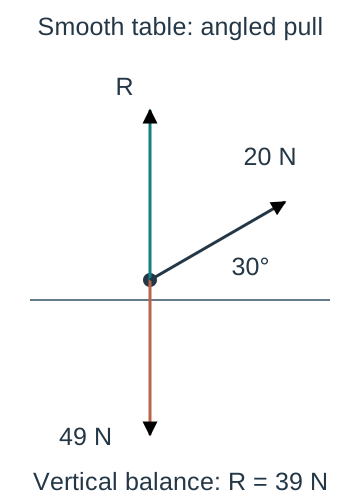
Angled pull and normal force — For mass 5 kg pulled by 20 N at 30° above horizontal with no vertical acceleration, upward pull is 10 N, so R+10−49=0 and R=39 N. The horizontal pull is 10√3 N. Ignoring the upward component would overestimate the contact force and any friction based on it.
For a five-kilogram body and g=9.8, the applied twenty-newton force is thirty degrees above horizontal, giving upward component ten and required reaction thirty-nine newtons under zero vertical acceleration. The point diagram displays the actual three forces on the smooth-table body. Force arrow lengths are schematic, while the applied direction uses the stated thirty-degree geometry; no friction is asserted in this smooth illustration.
Angled push comparison — If the same 20 N is directed 30° below horizontal, its vertical component is downward and R=49+10=59 N while horizontal component remains 10√3 N. The push can increase available friction. State the direction explicitly rather than treat an unsigned angle as sufficient information.
Loss of contact — A nonadhesive surface reaction must be nonnegative. If an assumed contact equation requires R<0, the surface would have to pull, so the constrained-contact model fails; use R=0 at detachment and model subsequent free motion appropriately. A very strong upward force need not leave a body sitting on the table.
Vertical lift equation — For a passenger of mass m with upward-positive acceleration a, normal force N satisfies N−mg=ma. Thus N=m(g+a). If acceleration is downward with magnitude b, use a=−b, giving N=m(g−b) while contact remains valid. Direction of motion alone does not determine the sign of acceleration.
Lift at constant velocity — A lift travelling upward or downward at constant velocity has a=0, so N=mg for the passenger under the simple model. During upward acceleration N is greater than mg and during downward acceleration it is less. Apparent support force changes while the passenger's mass does not.
Free fall and support — In the ideal free-fall case a=−g, the contact expression gives N=0, describing no supporting normal force. Weight mg still acts; apparent weightlessness is not the absence of gravity. A model requiring a downward support force from a simple floor cannot maintain that same contact.
Two bodies in vertical contact — For a fictional upper block of 3 kg on a lower block of 2 kg, both accelerating upward at 2 m/s², the contact force supporting the upper block is 3(9.8+2)=35.4 N. An external upward force supporting both must be 5(9.8+2)=59 N if it is the only such force. Separate diagrams identify which mass belongs in each equation.
Changing stages — A connected or contact system may change when a string becomes slack, a body reaches the floor or contact is lost. Solve each valid interval with its own forces and constraints; velocities at transition can supply initial conditions for the next stage. A previously derived common acceleration does not persist automatically after an interaction disappears.

Friction limiting equilibrium and rough-plane motion

Friction direction — Friction opposes actual sliding or the tendency to slide relative to the contact surface. In a stationary problem determine the impending motion tendency before choosing its direction. Friction is not always opposite the body's absolute velocity, for example when comparing a moving contact surface with the body.
Static friction inequality — For a simple rough-contact model in equilibrium, friction magnitude F satisfies 0≤F≤μR. It adjusts to the tangential force needed for equilibrium up to that bound. Do not set F=μR automatically for every stationary body; equality applies at limiting equilibrium or an explicitly modelled sliding stage.
Coefficient of friction — The parameter μ is nonnegative and dimensionless. In this course's ideal sliding model, friction magnitude is μR while the direction opposes sliding. Real surfaces may have more complex behaviour; identify the simplified law specified rather than import an unprovided speed-dependent law.
Stationary horizontal example — A 5 kg body on a horizontal surface with μ=0.3 has R=49 N and limiting friction 14.7 N. If a horizontal 10 N pull is applied and the body can remain at rest, actual friction is 10 N, not 14.7 N. Equilibrium fails when the required friction exceeds the available bound.
For the fictional five-kilogram body with μ=0.3 and R=49, equilibrium friction follows the required horizontal applied pull until its limiting value 14.7 N. Both axes use 15 pixels per newton with origin (60,400). The green line ends at that limit; no continuation or kinetic-friction curve is claimed beyond it. The horizontal brown reference marks available limiting friction, not the actual friction for every pull.
Limiting equilibrium — A body just about to slip has the friction magnitude at μR in the direction opposing that impending motion. Use the equality together with resolved force equations. If more than one direction of impending slip is possible, examine each limiting case instead of assuming a single friction sign for all applied forces.
Rough horizontal motion — For a 5 kg body sliding right under horizontal pull 20 N with μ=0.2, R=49 N, friction is 9.8 N left and acceleration is (20−9.8)/5=2.04 m/s² right. This assumes it is already sliding right under the stated model; initial rest would first require a check against limiting static friction.
Angled rough-plane pull — For the earlier 20 N pull at 30° above horizontal and mass 5 kg, R=39 N. With μ=0.2 and sliding right, friction is 7.8 N and acceleration (10√3−7.8)/5≈1.9041 m/s². The normal equation and friction law are coupled through the angled force.
Weight on an incline — On a slope at angle θ above horizontal, weight has downslope component mg sinθ and into-plane component mg cosθ. Resolve parallel and normal to the plane. These are components of one weight force, not two additional weights to add alongside mg in the same diagram.
Smooth incline motion — For a particle on a fixed smooth incline with no other normal forces, R=mg cosθ and downslope acceleration g sinθ. If the particle is projected uphill, its acceleration is still downslope while its uphill velocity decreases. The reaction is less than mg on an ordinary nonvertical incline.
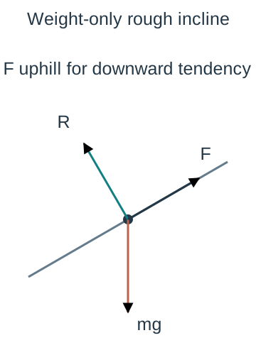
Equilibrium on a rough incline — With only weight, reaction and friction on a fixed incline, equilibrium requires uphill friction mg sinθ and R=mg cosθ. The inequality becomes tanθ≤μ for 0≤θ<90° with ordinary contact. At limiting downward slip μ=tanθ; mass cancels and no arbitrary m remains in the coefficient.
The point-body diagram shows the three actual forces for a weight-only rough incline with downward sliding tendency: vertical weight, perpendicular reaction and uphill friction. The line is drawn at thirty degrees to horizontal, but force arrow lengths are schematic. The related note resolves the single weight into components algebraically rather than drawing those as extra physical forces.
Sliding down a rough incline — Under the course's μR sliding law and positive downslope axis, a=g(sinθ−μcosθ). A negative answer for an initially downslope-moving body means acceleration uphill and deceleration, not automatically an impossible stage. Check whether the motion stops and whether the subsequent static model permits rest or reversal.
Worked incline — For θ=30°, μ=0.2 and g=9.8, a=4.9−0.98√3≈3.2026 m/s² downslope. For a 5 kg body R=24.5√3 N and friction is 4.9√3 N uphill. Exact expressions retain the geometric factors before rounding.
Projected uphill with friction — For a particle moving uphill under only gravity and rough contact, both the downslope weight component and friction point downhill. With uphill-positive axis, a=−g(sinθ+μcosθ) while that sliding stage lasts. If it stops, reassess friction direction and the equilibrium inequality rather than keep the downhill-sliding expression unchanged.
Additional slope forces — A string or applied force at an angle to the plane can alter both tangential driving force and normal reaction. Resolve it into the slope axes before using μR. Setting R=mg cosθ is justified only when no additional normal component or normal acceleration changes that equation.
Friction feasibility — After solving a proposed static configuration, check the required |F|≤μR and R≥0. A calculated negative signed tangential friction can simply mean the actual direction is opposite the provisional arrow, while a negative magnitude μ or nonadhesive reaction is not an admissible result. Distinguish signed components from physical magnitudes.

Connected particles strings pulleys and system equations

Ideal pulley and string — A light taut inextensible string passing over an ideal smooth pulley is modelled with common tension and linked acceleration magnitudes in the simple arrangements considered. The pulley redirects the string; it does not make the attached bodies' acceleration vectors identical. Explain which constraint supplies each equality.
Separate particle equations — Draw a separate free-body diagram for each body and choose a positive direction along its expected motion. Write its own resolved ΣF=ma, using that body's mass. Connect the equations with common tension and acceleration only while the stated string and contact assumptions hold.
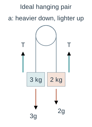
Hanging unequal masses — For fictional hanging masses 3 kg and 2 kg joined over an ideal pulley, choose the heavier body downward and lighter upward with common a. Equations are 3g−T=3a and T−2g=2a. Adding gives a=g/5=1.96 m/s² and then T=23.52 N for g=9.8.
The ideal pulley joins masses three and two kilograms by a light taut inextensible string. Each mass has upward tension T and downward weight of its own magnitude. The heavier body accelerates downward while the lighter accelerates upward with equal magnitudes under the constraint; arrows beside the string label forces, not acceleration. Body dimensions and force lengths are schematic.
Interpreting system addition — Tension cancels when adding those path-signed scalar equations because it is internal to the combined ideal system with matched constraints. This is not a claim that both bodies' spatial acceleration vectors point the same way. Solving the system total gives acceleration; return to a separate-body equation to recover tension.
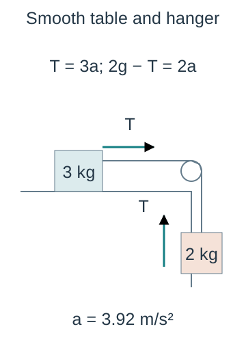
Table and hanging mass — A 3 kg body on a smooth horizontal table connected to a hanging 2 kg mass has equations T=3a and 2g−T=2a. Thus a=2g/5=3.92 m/s² and T=11.76 N under the ideal string/pulley model. The table body has vertical reaction 3g because its tension is horizontal in this geometry.
The geometry schematic connects a three-kilogram smooth-table body to a hanging two-kilogram mass. Horizontal tension accelerates the table body while hanging weight minus tension accelerates the second. The displayed force equations use each body mass separately. This is a constraint schematic rather than a complete free-body diagram: the table body vertical weight and reaction must also appear in its full separate diagram.
Rough table version — If that table contact has μ=0.2 and motion is towards the pulley, resistance is 0.2×3g=5.88 N. Equations T−5.88=3a and 19.6−T=2a give a=2.744 m/s² and T=14.112 N. First check the assumed motion or limiting equilibrium if the system begins from rest.
Connected inclined body — For a body on an incline linked to a hanging mass, resolve its weight along the plane and include friction with the actual motion tendency. Choose compatible path directions and preserve the string length constraint. Test both a proposed motion direction and an equilibrium possibility where the question requires it.
Contact-force pairs — When two particles remain in contact, their mutual force pair acts on different bodies and cancels only in a suitable combined-system equation. The force needed to accelerate one body is not generally the total driving force on both. Recover the contact magnitude from the body with the simplest complete force list.
Slack or impact stage change — If a hanging body reaches the floor, its previous motion constraint may cease and tension can change or vanish. Use the velocity just before transition only as a valid initial condition where the next-stage model allows it. Do not continue the old common-acceleration solution across an impact or slack string without stating new assumptions.

Force-model checks and connected explanations

Checking force equations — Verify each term is a force in newtons, the selected body and positive direction are stated and each acceleration component matches the geometry. Inspect whether the answer approaches the correct smooth, zero-force or equal-mass case when a parameter changes. A dimensionally correct equation can still have the wrong force signs or body mass.
Model limitations — Light strings, smooth pulleys, point particles, constant g and the μR friction law simplify a specific interaction. A massive string, rough pulley, stretching cord, tipping object or varying resistance may require different equations or constraints. Explain which claimed equality fails rather than only list generic real-life complications.
Communicating a physical solution — Present diagrams, signed component equations, constraints, solved values with units and checks on contact, tension, friction and stage validity. If a provisional direction produces negative acceleration, interpret it relative to that axis and actual velocity. Do not change signs to obtain a preferred narrative without rechecking the model.

Test yourself

50 questions · Random sets of 10. These quick checks support revision; practise longer explanations and justified judgements too.