Function definitions domains composites and inverses
Function rule — A function assigns exactly one output to each permitted input. Its domain is the set of permitted inputs and its range is the set of outputs actually obtained. Specifying f(x) = x² without stating a domain can leave an inverse or range question incomplete; over all real inputs its range is y ≥ 0.
Domain and restrictions — For f(x) = 1/(x − 3), exclude x = 3. For real g(x) = √(x + 2), require x ≥ −2. If expressions are combined, every component and the combined operation must be defined. A calculator returning a value for some inputs does not establish an unrestricted real domain.
One-to-one and many-to-one — A one-to-one function gives different outputs for different inputs. A many-to-one function can give the same output for distinct inputs while remaining a function: x² gives 4 at both −2 and 2. A horizontal line meeting a graph twice shows it is not one-to-one on the displayed domain.
Composite order — The notation fg(x) means f(g(x)): apply g first, then f. If f(x) = 2x + 1 and g(x) = x², then fg(x) = 2x² + 1 while gf(x) = (2x + 1)². Composition is generally not commutative, meaning the order matters, so reversing the order changes the rule and can change the domain.
Composite domains — For f(u) = √u and g(x) = x − 2, fg(x) = √(x − 2) requires x ≥ 2 because g(x) must lie in f's domain. For gf(x) = √x − 2, require x ≥ 0 instead. A composite input must be allowed by the inner function and its resulting output allowed by the outer one.
Range reasoning — For f(x) = (x − 3)² + 2 over all real x, the square is at least zero, so the range is y ≥ 2 with equality at x = 3. On the restricted domain x ≥ 4, the range becomes y ≥ 3. Use the actual allowed inputs rather than automatically read the unrestricted turning point as attainable.
Inverse meaning — An inverse function reverses a one-to-one correspondence between an original domain and its range. The notation f⁻¹(x) means inverse function, not 1/f(x). If f(x) = 3x − 5 on the real numbers, write y = 3x − 5 and solve x = (y + 5)/3, giving f⁻¹(x) = (x + 5)/3.
Checking an inverse — Check f(f⁻¹(x)) = x on f's range and f⁻¹(f(x)) = x on f's domain. For f(x) = 3x − 5, substitution into either composite recovers x. State the relevant sets, especially when a square root, logarithm or denominator restricts the original function.
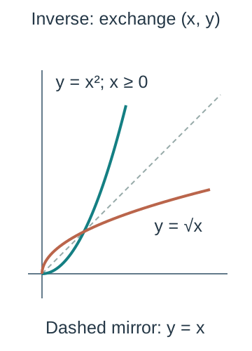
Restricting for an inverse — The function f(x) = x² has no inverse function on all real inputs because an output such as 4 would need two outputs under reversal. Restricting to x ≥ 0 gives inverse √x; restricting instead to x ≤ 0 gives inverse −√x. An inverse question therefore needs the chosen branch, not an automatic plus-or-minus expression.
Inverse graph — The graph of y = f⁻¹(x) is the reflection of y = f(x) in y = x, with each (a,b) becoming (b,a). Domain and range exchange roles. Reflect the stated restricted branch rather than the whole unrestricted curve when only one branch has an inverse.The nonnegative branch y=x² (green) and its inverse y=√x (brown) are reflected in the dashed line y=x. The plotted segments use equal scales of 60 pixels per unit on both axes. The full square function has domain x≥0 and range y≥0; the drawn segments illustrate part of those graphs rather than imposing finite domain endpoints.
Equations and intersections — The equation f(x) = g(x) asks for x-values where the two graphs have the same height. To solve x² = 2x + 3, intersections occur at x = −1 and 3, with paired coordinates (−1,1) and (3,9). A graphical estimate should be checked algebraically when an exact solution is requested.
Polynomial reciprocal and modulus graphs
Sketch versus plot — A sketch shows the important shape and labelled features without pretending every pixel is a measured value. Identify axes, intercepts, roots, asymptotes and relevant turning behaviour. Mark any domain restriction and avoid joining separate branches across a discontinuity, a break or jump in the function's values. A precise plotted graph additionally needs appropriate scales.
Cubic roots and end behaviour — For y = (x + 1)(x − 1)(x − 2), roots are −1, 1 and 2 and the y-intercept is 2. The leading coefficient is positive, so y tends to negative infinity as x tends to negative infinity and positive infinity as x tends to positive infinity. Use signs between roots to sketch the crossings.
Repeated polynomial roots — For y = x²(2x − 1)², both roots 0 and 1/2 have even multiplicity (each factor occurs twice) and the value is nonnegative everywhere. The graph touches the axis at each rather than changing sign there. Its leading term is 4x⁴, so both ends rise; the two factors do not imply only two-degree behaviour.
Odd and even multiplicity — A real polynomial changes sign through a root of odd multiplicity and retains its sign through a root of even multiplicity. A triple root can cross with a flattened shape. These local facts combine with the leading term and other roots; they do not alone locate every stationary point.
Reciprocal graph — For y = 1/x, the domain excludes zero, the axes x = 0 and y = 0 are asymptotes, lines that the graph approaches in the relevant limiting direction, and the branches lie in quadrants one and three. The value never equals zero. The graph approaches an asymptote without acquiring a missing input or output.
Reciprocal-square graph — For y = 1/x², x = 0 is excluded, y is always positive, and the graph is symmetric in the y-axis. Both branches rise without bound near x = 0 and tend to zero for large magnitudes of x. Unlike 1/x, negative inputs still give positive outputs.
Shifted reciprocal — For y = 2/(x + 3) − 1, the vertical asymptote is x = −3 and the horizontal asymptote is y = −1. The x-intercept is −1 and the y-intercept is −1/3. Identify the zero denominator and limiting constant rather than read the inner plus sign as a shift right.
Asymptote qualification — An asymptote describes limiting behaviour; it is not a universal assertion that every curve can never cross any asymptote. The simple reciprocal family a/(x − h) + k with nonzero a does not cross its horizontal asymptote k. Other rational curves can cross a horizontal asymptote elsewhere while still approaching it at infinity.
Modulus as magnitude — The modulus of a real number is its nonnegative magnitude: for x ≥ 0 it is x and for x < 0 it is −x. The graph y = modulus of x is V-shaped with vertex (0,0). Modulus is not the instruction to delete every minus sign wherever it appears in an expression.
Linear modulus graph — For y = modulus of (2x − 1), the vertex is at x = 1/2 where the inner expression vanishes. On x ≥ 1/2 the rule is 2x − 1; on x < 1/2 it is 1 − 2x. The output is nonnegative on both branches, and the y-intercept is 1.
Modulus equation — To solve modulus of (2x − 1) = x, the right side requires x ≥ 0. On x ≥ 1/2 solve 2x − 1 = x, giving 1. On 0 ≤ x < 1/2 solve 1 − 2x = x, giving 1/3. Both satisfy the original equation; the two branches correspond to different intersections.The green graph y=|2x−1| intersects the brown line y=x at x=1/3 and x=1, marked by the two dark dots in that order from left to right. Both axes use fixed scales within the plot (90 pixels per horizontal unit and 60 per vertical unit). The graph is above the line outside the crossings, giving the strict inequality solution x<1/3 or x>1. Labels below the plot identify the crossing x-values rather than additional plotted points.
Modulus inequality — For modulus of (2x − 1) > x, every x < 0 works because the left side is nonnegative. On the remaining branches, the solution is x < 1/3 or x > 1. Equality at 1/3 and 1 is excluded. A sketch with the line y = x makes the outside intervals visible.
Absolute-value intervals — For a > 0, modulus of (x − c) < a means c − a < x < c + a. It describes distance less than a from c. With modulus greater than a, the solution lies outside that interval. If the proposed right side is negative, reason from nonnegativity before applying an interval rule.
Graph transformations and composite changes
Vertical translation — The graph y = f(x) + a moves every point (x,y) to (x,y + a). Thus y = x² + 3 has vertex (0,3). The input remains unchanged; shifting a graph upward does not replace x by x + a in the rule.
Horizontal translation — The graph y = f(x + a) moves every point left by a when a is positive. The point with original input u now occurs at x = u − a, because x + a = u. Hence y = (x + 3)² has vertex (−3,0), not (3,0).
Vertical scaling — For y = af(x), each (x,y) maps to (x,ay). Positive a greater than one stretches vertically; 0 < a < 1 compresses. A negative a also reflects in the x-axis. With a = 0 the output is identically zero on the inherited input domain and should be treated separately.
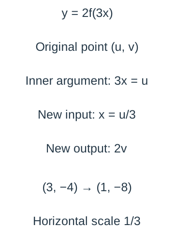
Horizontal scaling — For y = f(ax) with a ≠ 0, each original point (u,v) maps to (u/a,v). Thus f(3x) has horizontal scale factor 1/3. A negative a also reflects in the y-axis. Do not multiply the input coordinate by a when the multiplier appears inside the function.
Reflections — The graph y = −f(x) reflects in the x-axis, while y = f(−x) reflects in the y-axis. The first changes output sign; the second changes input sign. A function that happens to be even can look unchanged under the second reflection, but the transformation rule remains distinct.
Output modulus — To draw y = modulus of f(x), keep all portions with nonnegative y and reflect negative portions in the x-axis. Zeros stay zeros and the new range is nonnegative. This operation differs from replacing the input with its modulus, which instead copies the original right-hand branch onto the left.
Reflected output modulus — To draw y = modulus of f(−x), first reflect the original graph in the y-axis and then reflect any part below the x-axis upward. Test an actual point to check signs. Modulus after a reflection acts on output values, not on the variable's position.
Combined scaling — For y = 2f(3x), a point (u,v) becomes (u/3,2v). If f has a root at 6, the transformed root is 2; if (3,−4) lies on f, then (1,−8) lies on the transformed graph. Working through coordinates avoids a vague instruction to stretch both axes by the displayed numbers.For y=2f(3x), set the inner argument equal to an original input u, so x=u/3; multiply its corresponding output v by two. Thus an original point (3,−4) maps to (1,−8). The diagram tracks coordinates and does not depict distances on a graph.
Translation and reflection order — For y = f(−x) + 1, reflect in the y-axis then move up one. By contrast y = f(−(x + 1)) moves the reflected graph left one. Order matters when transformations affect the same coordinate; write a coordinate map or solve the inner argument rather than apply memorised words blindly.
General point mapping — For y = A f(B(x − h)) + k with B ≠ 0, a point (u,v) on f maps to (h + u/B, k + Av). State whether A is zero and how the domain changes. This formula follows by setting B(x − h) = u, so it can be derived rather than treated as a new unexplained rule.
Transforming restricted domains — If f is defined only for 1 ≤ u ≤ 4, then f(2x − 1) requires 1 ≤ 2x − 1 ≤ 4, so 1 ≤ x ≤ 5/2. A translated or scaled graph inherits a transformed domain. Do not draw an infinite curve if the original input interval was finite.
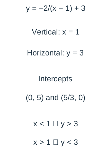
Transformed reciprocal example — For y = −2/(x − 1) + 3, start with 1/x, move right one, reflect and scale outputs by −2, then move up three. The asymptotes are x = 1 and y = 3; the intercepts are (0,5) and (5/3,0). The graph lies above the horizontal asymptote for x < 1 and below it for x > 1.The transformed reciprocal has vertical asymptote x=1 and horizontal asymptote y=3, with intercepts (0,5) and (5/3,0). The sign of −2/(x−1) places the left branch above y=3 and the right branch below it. These are derived features, not a plotted curve.
Rational expressions and partial fractions
Partial-fraction purpose — Partial fractions rewrite a rational expression, a fraction of polynomials, as a sum of simpler fractions on its original domain. The decomposition is an identity, not an equation holding only at a few selected x-values. It supports later integration, differentiation and series work, but cancellation or rearrangement never restores an excluded denominator zero.
Degree check — If the numerator degree is at least the denominator degree (degree means the highest power of the variable in a polynomial), perform algebraic division before using a proper-fraction template. For (x² + 1)/(x − 1), the result x + 1 + 2/(x − 1) includes a polynomial part. A sum with only constant numerators over the original linear factors may otherwise be incapable of matching the growth at infinity.
Distinct linear factors — Write (3x + 1)/((x + 1)(x − 1)) = A/(x + 1) + B/(x − 1). Clearing denominators gives 3x + 1 = A(x − 1) + B(x + 1). Substitution at 1 and −1, or coefficient comparison, yields A = 1 and B = 2. The original expression remains undefined at both inputs.
Substitution after clearing — Putting a root into the cleared polynomial identity determines a coefficient; it does not evaluate the original undefined fraction at that input. In the preceding example x = 1 gives 4 = 2B in an identity valid as a polynomial relation. Keep this distinction explicit when explaining the cover-up shortcut.
Comparing coefficients — From 3x + 1 = A(x − 1) + B(x + 1), equate x coefficients to get A + B = 3 and constants to get −A + B = 1. Solve to obtain A = 1 and B = 2. Equality of polynomials for every x justifies matching corresponding coefficients.
Nonmonic factors — Nonmonic means a factor's leading coefficient is not 1, as in 2x − 1. For (5x + 1)/((2x − 1)(x + 2)), write A/(2x − 1) + B/(x + 2). The cleared identity is 5x + 1 = A(x + 2) + B(2x − 1), giving A = 7/5 and B = 9/5. Remember that the root of 2x − 1 is 1/2; ignoring its coefficient changes the decomposition.
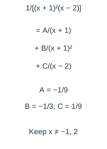
Repeated linear factor — A factor (x + 1)² requires both A/(x + 1) and B/(x + 1)², along with any other factor term. For 1/((x + 1)²(x − 2)), use those two terms plus C/(x − 2). Omitting the first power of the repeated factor can prevent an identity even when selected substitutions appear successful.
Repeated-factor working — Clearing the preceding denominator gives 1 = A(x + 1)(x − 2) + B(x − 2) + C(x + 1)². At x = −1, B = −1/3; at x = 2, C = 1/9. Comparing x² coefficients gives A + C = 0, so A = −1/9. Check by recombining the fractions on x ≠ −1,2.The complete repeated-factor decomposition is −1/[9(x+1)]−1/[3(x+1)²]+1/[9(x−2)], retaining x not equal to −1 or 2. Both first and second denominator powers are necessary. The notes derive each coefficient from the cleared identity and explain why substituting excluded roots there does not define the original fraction.
Three distinct terms — For 1/(x(x − 1)(x + 1)), write A/x + B/(x − 1) + C/(x + 1). The cleared identity gives A = −1, B = 1/2 and C = 1/2. Three denominator factors require a complete template, not a guessed two-term expression.
Recombination check — Combine a proposed decomposition over the original common denominator and compare the whole numerator symbolically. A few numerical checks can catch mistakes but cannot by themselves establish an identity. In repeated-factor work, verify both the coefficient values and the presence of every required denominator power.
Scope and later use — For this course the assessed decomposition denominators use linear factors with powers no more than squared, no more than three terms, and constant or linear original numerators. General irreducible-quadratic templates are not required here. Algebraic division can first produce a proper rational part; later chapters apply the same identities with their original restrictions.
Proportion and evaluating function models
Direct proportion — If y is directly proportional to x, write y = kx with constant k. A graph of y against x passes through the origin within the mathematical model, and y/x is constant for nonzero x. An arbitrary straight line y = mx + c with c ≠ 0 does not express direct proportion between y and x.
Inverse proportion — If y is inversely proportional to x, write y = k/x for x ≠ 0, so xy = k. Doubling a nonzero input halves the output when k is fixed. In a physical context, positivity or other limits may restrict the domain to one reciprocal branch rather than every mathematically allowed real x.
Power proportion — If y is proportional to x², write y = kx². For positive inputs, doubling x multiplies y by four. Plotting y against x² gives a straight line through the origin if the model holds, whereas y against x is generally curved. Keep track of which quantity is plotted on each axis.
Calibrating a model — If pressure P is modelled as k/V for a fixed amount of gas at constant temperature, data P = 120 kPa at V = 0.8 m³ give k = 96 kPa m³. At V = 1.2 m³ the model gives 80 kPa. State the fixed conditions, compatible units and positive-volume domain rather than imply an unconditional physical law for every experiment.
Checking model fit — One observation can determine k but cannot establish that the proportional relationship is valid throughout a range. Test other observations, inspect deviations and consider measurement uncertainty and omitted influences. A graph or transformed plot can reveal a pattern while still needing contextual judgement about why the model might apply.
Extrapolation and refinement — A function fitted over one range may fail outside it. A population cannot grow exponentially without resource limits indefinitely, and a reciprocal physical model may be meaningless at zero input. State plausible domain restrictions and suggest a justified refinement linked to actual discrepancies, rather than assume a more complicated formula is always better.
Interpreting solutions — After solving a mathematical model, translate the answer into the original quantities with units and a sensible precision. Reject roots outside the physical domain and explain why. An algebraically valid input may still be excluded by the original modelling assumptions, so solving an equation is one step within the modelling cycle.
Test yourself
50 questions · Random sets of 10. These quick checks support revision; practise longer explanations and justified judgements too.
 Mr Kidman's Classroom