Antiderivatives definite accumulation and the fundamental theorem
Integration as reversal — An antiderivative F of f satisfies F′(x)=f(x) on a specified interval. An indefinite integral represents the family F(x)+C because differentiating any constant gives zero. The symbol ∫ denotes integration and dx identifies x as the variable of integration. For ∫2x dx, the result is x²+C, not one uniquely determined curve until additional information selects C.
The integration constant — Keep +C in a general indefinite result, including when the integrand, the function being integrated, is zero. Separate disconnected intervals can have independently chosen constants; an antiderivative formula does not force continuity across an excluded denominator zero. A definite integral instead evaluates a number and does not retain an arbitrary +C.
Recovering a curve — If dy/dx=6x−4, then y=3x²−4x+C. Given y=5 at x=1, substitution gives C=6, so y=3x²−4x+6. Use the original function-value condition after integrating rather than insert it into the derivative as though it determined the missing constant directly.
Definite integral — The notation ∫ from a to b of f(x) dx denotes signed accumulated change over the interval. Under the usual continuous-integrand conditions, an antiderivative gives ∫f=F(b)−F(a). Evaluate at both complete bounds, including every term and its sign.
Fundamental theorem — For continuous f, differentiating the accumulated function G(x)=∫ from a to x of f(t) dt gives G′(x)=f(x). Together with antiderivative evaluation, this connects local rate and accumulated change. The integration variable t is dummy; the upper bound x is the variable of the resulting function.
Limit of sums — Partition [a,b] into n equal widths Δx=(b−a)/n and choose a point xᵢ in each strip. The sum Σ f(xᵢ)Δx approximates signed accumulation; for continuous f it approaches the definite integral as the maximum strip width tends to zero. Negative heights contribute negatively rather than become positive automatically.
A sum-limit example — For ∫ from 0 to 1 of x dx, right endpoints are i/n and width 1/n. The sum is (1/n²)Σ from i=1 to n of i=(n+1)/(2n), which tends to 1/2. Finite right rectangles overestimate this increasing positive line, while their limit equals the exact triangular area.For f(x)=x on [0,1], four right-endpoint rectangles have total 5/8, above the exact integral 1/2. Their widths are one quarter and heights one quarter, one half, three quarters and one. The horizontal scale is 240 pixels per input unit and vertical scale 220 per output unit. Increasing n produces the sum (n+1)/(2n), whose limit is one half.
Bounds and splitting — Reversing bounds reverses sign: ∫ from b to a of f is minus ∫ from a to b of f. Integrating from a point to itself gives zero. A definite integral can be split at an intermediate point c as the sum over [a,c] and [c,b], useful for sign changes or different expressions.
Linearity and units — Definite and indefinite integration distribute over sums and fixed scalar multipliers. A rate with units metres per second integrated with respect to seconds gives displacement in metres. An area interpretation requires identifying the axes; not every integral represents a physical area with length squared units.
Conditions before evaluation — Check that the integrand and interval justify ordinary antiderivative evaluation. The expression 1/x is undefined at zero, so its integral across an interval containing zero cannot be treated as a single continuous proper integral and declared zero from matching logarithm endpoints. Handling singular improper integrals is a separate issue, not an excuse to ignore a pole, an undefined input near which the function grows without bound in magnitude.
Standard integrals powers exponentials logarithms and trig identities
Power integration — For rational n with n≠−1, ∫xⁿ dx=xⁿ⁺¹/(n+1)+C on an appropriate real interval. Increase the exponent by one and divide by that new exponent. The exception n=−1 would create a zero denominator and needs a logarithm instead.
Radicals and negative powers — For x>0, ∫√x dx=(2/3)x³ᐟ²+C and ∫x⁻² dx=−x⁻¹+C on intervals excluding zero. Rewriting a radical or reciprocal as a power clarifies which rule applies. Preserve the original real domain when simplifying an integrand.
Algebra first — Expand or divide before integrating where that creates standard powers. For (x+1)²/√x on x>0, the integrand is x³ᐟ²+2x¹ᐟ²+x⁻¹ᐟ², giving (2/5)x⁵ᐟ²+(4/3)x³ᐟ²+2√x+C. Differentiate the result to check every exponent and coefficient.
The one-over-x exception — The integral of 1/x is ln|x|+C on an interval excluding zero. For x>0 this is ln x+C, while negative intervals need ln(−x)+C. A logarithm of a negative argument without the magnitude is not a real antiderivative there.
Linear denominator — For a≠0, ∫1/(ax+b) dx=(1/a)ln|ax+b|+C, excluding the denominator root. Thus ∫3/(5x+2) dx=(3/5)ln|5x+2|+C. The factor 1/a is necessary because differentiating the logarithm multiplies by a.
Exponential integrals — For nonzero k, ∫eᵏˣ dx=eᵏˣ/k+C. A constant multiplier remains outside, and an additive exponent constant is retained. If k=0 the integrand is one and the result x+C, so do not divide by k at zero.
General exponential base — For a>0 and k ln a nonzero, ∫aᵏˣ dx=aᵏˣ/(k ln a)+C. If a=1 or k=0 the integrand is constant one instead. This follows from the derivative's logarithmic base factor rather than a new unrelated rule.
Sine and cosine integrals — For nonzero k with radian inputs, ∫sin(kx) dx=−cos(kx)/k+C and ∫cos(kx) dx=sin(kx)/k+C. Differentiate to verify the minus sign and reciprocal scale. A zero k gives a constant integrand and is handled directly.
Squared secant — For k≠0, ∫sec²(kx) dx=tan(kx)/k+C on each interval where cosine is nonzero. In particular ∫sec²(2x) dx=(1/2)tan(2x)+C. The coefficient reverses the inner derivative factor; it is not a multiplication by two.
Tangent integral — Since tan x=sin x/cos x, ∫tan x dx=−ln|cos x|+C where cosine is nonzero. Differentiate this logarithm to check the sign. The antiderivative is valid on separate intervals between tangent asymptotes, not across an undefined input as one continuous proper integral.
Squared sine and cosine — Use sin²x=(1−cos 2x)/2 to get ∫sin²x dx=x/2−sin 2x/4+C. Similarly ∫cos²(3x) dx=x/2+sin 6x/12+C. Integrating a squared trig output does not follow the polynomial power rule applied to the function's name.
Tangent squared — From tan²x=sec²x−1, ∫tan²x dx=tan x−x+C on its domain. An identity can turn a nonstandard-looking integrand into known pieces. Retain the original denominator exclusions and check by differentiation rather than assume the same formula applies at an asymptote.
Checking an indefinite result — Differentiate a proposed antiderivative and compare it with the original integrand on the stated domain. This catches missing constants of scale, incorrect signs and algebraic simplifications. Two antiderivatives with derivatives equal on a connected interval differ by a constant, so their appearances can differ without either being wrong.
Definite integrals signed area and parametric regions
Evaluating bounds — For ∫ from 1 to 3 of (2x+1) dx, use F=x²+x to obtain (9+3)−(1+1)=10. Bracket the whole lower-bound result before subtracting. A missing lower term or sign can change the answer even when the antiderivative is correct.
Integral versus total area — A definite integral combines positive and negative contributions. For ∫ from −1 to 1 of x³ dx, symmetry gives zero, but the total geometric area between the curve and axis is 1/2. Split at zero and add the magnitudes of the two signed quarter-unit areas.For y=x³ over [−1,1], the left contribution is −1/4 and the right contribution +1/4, so the signed integral is zero. The total geometric area adds their positive magnitudes to one half. Both axes use 120 pixels per coordinate unit. The coloured regions are split at the zero crossing, not combined before taking a magnitude.
Area with an axis — To find total area over a specified interval, locate every zero where the curve changes sign, split into subintervals and choose a positive area contribution on each. Taking the magnitude of the whole integral can hide cancellation and give an area that is too small.
Area between graphs — Find intersections and integrate upper function minus lower function over the correct x-interval. The integrand is their vertical separation. If the curves exchange order within a larger interval, split at the crossing; subtracting one fixed order across every part can cancel physical areas.
Parabola and line example — For y=6x−x² and y=2x, intersections are x=0 and 4. The parabola is above the line between them, so area is ∫ from 0 to 4 of (4x−x²) dx=[2x²−x³/3] from 0 to 4=32/3. The area is between the two graphs, not simply under the parabola.The shaded separation between y=6x−x² and y=2x extends from their intersections x=0 and x=4. Integrating upper minus lower gives ∫₀⁴(4x−x²)dx=32/3. Horizontal scale is 60 pixels per unit and vertical scale 25. The top curve is above the line throughout this particular enclosed region.
Two-curve example — For y=x²−5x+6 and y=4−x², intersections satisfy 2x²−5x+2=0, giving x=1/2 and 2. The second curve lies above the first there. Integrate −2x²+5x−2 between those bounds to obtain 9/8 square coordinate units, checking the exact fractional lower bound.
Regions with straight boundaries — A finite region may also include specified vertical or horizontal lines. Sketch and identify which graph forms each boundary before choosing bounds and integrands. An intersection outside the requested region does not automatically become an integration limit.
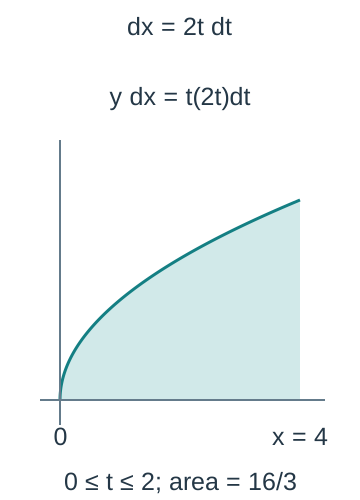
Parametric area relation — For x=x(t),y=y(t) with a suitable monotonic x-interval, ∫y dx=∫y(t)(dx/dt)dt using corresponding parameter bounds. The derivative factor converts parameter width into horizontal width. Simply integrating y(t) with respect to t generally calculates a different quantity.
Parametric area example — For x=t²,y=t with 0≤t≤2, the x-coordinate runs from 0 to 4 and dy is not the needed width. Area under the positive curve is ∫ from 0 to 2 of t(2t)dt=16/3. Eliminating t gives y=√x and confirms the same area over x from 0 to 4.With x=t²,y=t and 0≤t≤2, horizontal width is dx=2t dt, so the area integral is ∫₀²2t²dt=16/3. The plotted curve is y=√x from x=0 to 4, using horizontal scale 60 pixels per x unit and vertical scale 100 per y unit. The parameter upper bound two is not the x upper bound four.
Orientation and interpretation — If x decreases as the parameter increases, the signed ∫y dx follows that orientation; choose or reverse bounds consistently for the requested positive region. A loop or changing x-direction needs further splitting. State whether the answer is signed accumulation, total geometric area or a contextual quantity with its units.
Substitution as reverse chain rule
Choosing a substitution — A useful substitution identifies an inner expression u=g(x) whose derivative appears elsewhere in the integrand up to a constant. Replace every occurrence of x and the differential consistently so the new integral is entirely in u. The assessed simple cases require one suitable substitution, not an unexplained jump to an answer.
Differential relation — From u=g(x), write du=g′(x)dx to track the matching differential factor. For u=2x+1, dx=du/2. Omitting this half changes the answer even if the new power is integrated correctly; the notation summarises the chain-rule reversal.
Composite cosine example — For ∫2x cos(x²+1) dx, put u=x²+1 and du=2x dx. The integral becomes ∫cos u du=sin u+C, so the answer is sin(x²+1)+C. Differentiating confirms both the inner factor and the cosine.
Linear-root example — For ∫√(2x+1) dx on an appropriate real interval, let u=2x+1. Then (1/2)∫u¹ᐟ²du=(1/3)u³ᐟ²+C, giving (1/3)(2x+1)³ᐟ²+C. The original function and finite differentiability conditions still need the stated domain.
Rational composite example — For ∫x/(x²+4)² dx, take u=x²+4, so x dx=du/2. The result is (1/2)∫u⁻²du=−1/(2u)+C, hence −1/[2(x²+4)]+C. The denominator x²+4 stays positive for real x.
Log-derivative recognition — An integrand f′(x)/f(x) has antiderivative ln|f(x)|+C on a nonzero continuous-sign interval. For 2x/(x²+5), the denominator is positive, so ln(x²+5)+C suffices. The numerator must match the derivative of the entire denominator, not merely resemble it.
Trig substitution example — For ∫cos x√(1+sin x) dx, set u=1+sin x and du=cos x dx. Integrate to get (2/3)(1+sin x)³ᐟ²+C where the expression is real. This is a direct reverse-chain substitution; selecting u=cos x would not immediately supply the required differential in this form.
Definite substitution bounds — In ∫ from 0 to 1 of 2x ex²+1 dx, u=x²+1 changes the bounds to 1 and 2. Thus the integral is ∫ from 1 to 2 of eᵘdu=e²−e. Once the bounds are transformed, evaluate in u; do not put the old x bounds into the new antiderivative.The variable change u=x²+1 sends original x bounds zero and one to new bounds one and two. The factor 2x dx becomes du, leaving the exponential integral in u. Evaluate with those new bounds, or back-substitute fully before using old x bounds; mixing the two systems changes the answer.
Back-substitution alternative — For an indefinite result, return to the original variable unless a parametric answer is explicitly requested. For a definite integral, one may instead back-substitute before using the original bounds, but do not mix the two approaches. Both consistent methods give the same result.
Testing the choice — If a proposed substitution leaves unmatched x-dependence, reassess whether it actually simplifies the problem or solve for the remaining x expressions correctly. Inspect algebraic simplification and known derivative patterns first. A substitution name alone does not justify ignoring an inconvenient factor.
Integration by parts and repeated applications
Parts formula — Rearrange the product derivative (uv)′=u′v+uv′ and integrate to obtain ∫u v′ dx=uv−∫v u′ dx. In differential notation ∫u dv=uv−∫v du. Choose u so its derivative helps simplify the remaining integral and v′ so its antiderivative is known.
Polynomial-exponential example — For ∫x eˣ dx, choose u=x and v′=eˣ. Then u′=1,v=eˣ, so the result is xeˣ−∫eˣdx=(x−1)eˣ+C. Differentiating the product confirms that the extra exponential terms cancel.
Integrating a logarithm — For ∫ln x dx on x>0, choose u=ln x and v′=1, giving v=x. The formula gives x ln x−∫1 dx=x ln x−x+C. Treating the integral as a product with the constant function one reveals a useful parts choice.
Logarithmic product — For ∫x ln x dx with x>0, take u=ln x and v′=x. The answer is (x²/2)ln x−∫x/2 dx=(x²/2)ln x−x²/4+C. Differentiating checks the cancellation of the extra x/2 term.
Repeated parts — For ∫x²eˣ dx, the first application gives x²eˣ−2∫xeˣdx. Applying parts again yields eˣ(x²−2x+2)+C. Show both stages and avoid a formal reduction formula, which is outside the required scope here.A first parts application reduces ∫x²eˣdx to x²eˣ−2∫xeˣdx. A second application gives (x−1)eˣ for the remaining primitive, and the combined result is eˣ(x²−2x+2)+C. All intermediate arbitrary constants can be absorbed into the final one; the displayed final result is checked by differentiation.
Cyclic parts example — If I=∫eˣsin x dx, parts gives I=eˣsin x−∫eˣcos x dx. Applying parts to the remaining integral produces eˣcos x+I, so 2I=eˣ(sin x−cos x). Thus I=eˣ(sin x−cos x)/2+C; recognise and solve for the repeated original integral.
Definite parts — For definite bounds, include the boundary term [uv] from a to b and the remaining definite integral. For ∫ from 0 to 1 of xeˣ dx, [(x−1)eˣ] gives 0−(−1)=1. The antiderivative still comes from parts, but no arbitrary +C remains in the final number.
Rational integration and partial fractions
Simpler denominator first — For a rational integrand, inspect factorisation, division, a linear-denominator standard form or an f′/f pattern before choosing a longer method. For ∫4/(2x−1)² dx, reverse the chain-power derivative to obtain −2/(2x−1)+C. A squared linear denominator does not automatically demand logarithms.
Distinct-factor integral — The decomposition (3x+1)/((x+1)(x−1))=1/(x+1)+2/(x−1) gives antiderivative ln|x+1|+2ln|x−1|+C. Both x=−1 and x=1 remain excluded. Check the decomposition and the integral, since a correct method on wrong coefficients still gives a wrong answer.
Nonmonic-factor integral — For (5x+1)/((2x−1)(x+2)), use coefficients (7/5)/(2x−1)+(9/5)/(x+2). Integration gives (7/10)ln|2x−1|+(9/5)ln|x+2|+C. The first coefficient halves because its denominator derivative is two.
Repeated-factor integral — For 1/((x+1)²(x−2)), use −1/[9(x+1)]−1/[3(x+1)²]+1/[9(x−2)]. Integrating gives −(1/9)ln|x+1|+1/[3(x+1)]+(1/9)ln|x−2|+C. The first-power terms produce logs while the squared term produces a reciprocal.A first-power linear denominator gives a logarithm of magnitude, whereas its squared denominator gives a reciprocal-power antiderivative. Both expressions retain x≠−1. Repeated partial fractions therefore need term-by-term choice of rule rather than treating every denominator term as a logarithm.
Improper rational expression — Divide (x²+1)/(x−1) as x+1+2/(x−1) before integrating. The result is x²/2+x+2ln|x−1|+C on either interval excluding one. A proper-fraction template alone would miss the polynomial part.
Definite rational domains — Before evaluating a rational definite integral, identify every denominator zero in or at its interval. A correct partial-fraction antiderivative cannot justify ordinary endpoint subtraction across an internal pole. If the interval is valid, evaluate exact logarithm differences and retain signs through the original bounds.
Verification and equivalent logs — Differentiate the full result, recombine fractions and compare with the original rational function. Logarithmic laws can combine valid magnitude expressions on a fixed interval, so equivalent answers can look different. Do not remove magnitude or interval conditions merely to make an answer appear shorter.
Separable differential equations and solution families
Separation structure — For dy/dx=g(x)h(y), move y-dependent factors to the dy side and x-dependent factors to the dx side where division is valid. Integrate both sides and include one arbitrary constant in the combined relation. Check any zero of h(y) separately, because dividing by it can lose an equilibrium solution, a constant value of y that makes the original derivative zero for all relevant x.
Linear-in-y example — For dy/dx=2xy and y nonzero, separate dy/y=2x dx. Integration gives ln|y|=x²+C, so y=Aex², with sign determined by the initial condition. The separate equilibrium y=0 is included when A=0; it should be recovered explicitly after the division step.
Initial value in a solution — For that equation with y(0)=3, A=3 and y=3ex². Substitute back to verify y′=2xy and the initial value. A constant found from an initial condition selects one member of a family; it does not replace the need to check the differential equation itself.
Sketching the family — The family y=Aex² has a minimum at x=0 when A>0, a maximum there when A<0 and the x-axis when A=0. Members retain their sign and scale vertically. Use the explicit formula and derivative to sketch several solutions with labelled initial values rather than assume every solution is an ordinary eˣ growth curve.The curves y=exp(x²) and y=−exp(x²) have initial values 1 and −1; the horizontal axis is the A=0 solution. Horizontal scale is 80 pixels per input unit and vertical scale 50 per output unit. Positive A has a minimum at zero, negative A a maximum; these solution curves differ from an ordinary monotone eˣ graph.
Implicit separated result — For dy/dx=(x+1)/(y+2), require y≠−2 and separate (y+2)dy=(x+1)dx. Integration can be written (y+2)²=(x+1)²+C after absorbing constants. The implicit relation is useful, but an explicit branch must agree with any initial condition and the original denominator restriction.
Choosing the branch — With y(0)=1 in that example, C=8 and y+2 is positive initially. The selected solution is y=−2+√((x+1)²+8), which never reaches the forbidden value −2. Keeping an unjustified ± sign after using the initial condition would leave an extra incompatible family member.
Factoring before separation — For dy/dx=x y(y−1), equilibrium solutions y=0 and y=1 follow from the original equation. For the remaining branches, separate dy/[y(y−1)]=x dx and use −1/y+1/(y−1) for the left-hand fraction. Integrating gives ln|(y−1)/y|=x²/2+C on the valid branches.Both constant solutions y=0 and y=1 satisfy the original differential equation. The separated logarithmic relation is derived only for other branches because division by y(y−1) excludes those values. Restore equilibria explicitly and check which are represented after exponentiating and choosing constants.
Explicit non-equilibrium branch — Rearranging that relation gives y=1/[1−Aex²/2] where the denominator is nonzero. The constant y=1 is represented by A=0, while y=0 still needs the separate equilibrium branch. Verify by differentiation and retain any finite blow-up boundary, a finite input near which the solution magnitude grows without bound, rather than claim the same solution exists for all real x.
Domain from initial data — For y(0)=2 in the preceding equation, A=1/2 and the denominator vanishes at x=±√(2 ln 2). The continuous solution interval containing the initial input is between those two values. A formula that can be evaluated on another disconnected interval is not automatically a continuation through an undefined point.For y=1/[1−(1/2)exp(x²/2)], the initial point is (0,2). Denominator zeros at ±R, where R=√(2 ln 2), bound the connected solution interval (−R,R) containing zero. Dashed vertical lines show those boundaries; the curve continues unbounded beyond the plotted vertical viewport near them. Horizontal scale is 100 pixels per x unit and vertical scale 50 per y unit. Separate branches beyond a pole are not a continuous continuation through it.
Constant and verification discipline — One arbitrary constant is enough after integrating both sides because two separate additive constants can be combined. Exponentiation can absorb positive scale into a constant while an initial sign or a separately checked equilibrium must be preserved. Always check the original equation, initial value and connected domain, not just the separated algebra.
Contextual differential-equation solutions and limitations
Proportional growth solution — Solving dN/dt=kN gives N=Aeᵏᵗ, with A fixed by the initial amount. For an initial 200 and k=0.03 per time unit, N=200e0.03t. The formula satisfies the rate equation, but its indefinite increase is only as credible as the constant-rate and resource assumptions.
Approach to equilibrium — For dy/dt=−k(y−L), k>0, separation gives y=L+Ae⁻ᵏᵗ. With L=20 and y(0)=100, A=80. The equilibrium y=L is included by A=0 and should not be lost through division by y−L; nonzero A approaches L without reaching it at finite time.
Shrinking-radius solution — For dr/dt=−k/r² with r>0,k>0, integrate r²dr=−kdt to obtain r³=r₀³−3kt. The physical solution is r=(r₀³−3kt)¹ᐟ³ while 0≤t<r₀³/(3k). At zero radius the original rate law is undefined, so a negative real-cube-root extension is not a physical continuation.This illustrative case uses r₀=2 and k=1, giving r³=8−3t. Positive radius requires 0≤t<8/3. The open endpoint marks zero radius, where the original inverse-square rate law is undefined and the physical solution stops. Horizontal scale is 90 pixels per time unit and vertical scale 120 per radius unit; no negative-radius continuation is shown.
Volume interpretation — Combining that radius law with sphere volume 4πr³/3 gives dV/dt=−4πk, a constant volume loss rate while the model remains valid. The radius loss rate itself is not constant. This connection helps check dimensions and explain what the inverse-square radial law implies geometrically.
Kinematic initial conditions — If acceleration is a=6t, integration gives v=3t²+C. With v(0)=2, v=3t²+2; integrating again and using s(0)=5 gives s=t³+2t+5. Velocity and position need their own constants and initial conditions, and their units differ.
Long-time validity — A separated solution can predict indefinite growth, a limiting level or a finite singularity. Compare these with the physical setting and retain the allowed observation interval. A solution approaching a mathematical boundary does not prove the real process can continue under the same assumptions indefinitely.
Interpreting predictions — State what each solved variable measures, its units, the initial event and any sign or branch choice. Distinguish signed displacement from travelled distance and an ideal continuous count from exact discrete observations. Explain one concrete limitation and a justified possible refinement rather than treat a correct integration as proof that the model describes reality.
Test yourself
50 questions · Random sets of 10. These quick checks support revision; practise longer explanations and justified judgements too.
 Mr Kidman's Classroom