K5MA10 · Numerical roots iteration Newton–Raphson and trapezium estimates · Edexcel A-level Mathematics

Revise the key ideas

Root location continuity and certified accuracy

Root and residual — A root α of f satisfies f(α)=0. A numerical approximation x gives residual f(x), measuring how far the output is from zero rather than directly how far x is from α. State the original equation and allowed input domain before applying a numerical method.
Continuous sign bracket — If f is continuous on [a,b] and f(a),f(b) have opposite signs, at least one root lies between them. Continuity rules out a jump or pole masquerading as a zero. A sign bracket establishes existence, not uniqueness unless further reasoning is supplied.
Cubic bracket example — For f(x)=x³−x−2, f(1)=−2 and f(2)=4, so a root lies in (1, 2). Since f′(x)=3x²−1>0 throughout [1, 2], the function is increasing there and the bracketed root is unique. The derivative argument supplies information the sign change alone does not.
The cubic f=x³−x−2 is negative at one and positive at two, and it is continuous and strictly increasing on this interval. The plot therefore supports exactly one root between them. Horizontal scale is 240 pixels per input unit and vertical scale 35 per output unit; the horizontal line is y=0 and the viewport does not include the vertical axis x=0.
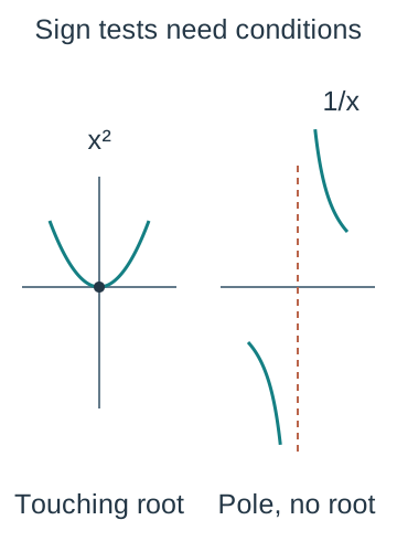
No sign change does not exclude a root — For f(x)=x², both f(−1) and f(1) are positive despite a root at zero. A repeated even-multiplicity root may touch the axis without crossing. Do not conclude that an interval contains no roots merely because its endpoint signs agree.
Wide interval failure — The function (x−1)(x−2) has two roots between zero and three, yet both endpoint values equal 2. An interval spanning an even number of crossings can have matching signs. Use a sketch, derivative information or smaller intervals rather than treat a single wide test as a complete root count.
Discontinuity failure — For f(x)=1/x, f(−1)<0 and f(1)>0 but no real input gives zero. The interval contains the pole at zero and the continuity condition fails. A numerical sign-change routine needs this domain check before claiming a root.
The left x² graph has a root at zero without a sign change. The right 1/x graph changes endpoint signs across zero but has a pole, not a root. Both panels use horizontal scale 45 pixels per input unit; vertical scales are 60 and 50 respectively. The dashed vertical line is the excluded pole; the branches are never joined across it.
Bisection step — For a continuous sign bracket, evaluate f at midpoint m=(a+b)/2 and retain the half still showing opposite signs; if f(m)=0 exactly, the root has been found. For the cubic bracket [1, 2], f(1.5)=−1/8, so the next bracket is [1.5, 2]. Each accepted update retains the sign evidence.
Further bisection — The next midpoint is 1.75, where the cubic value is 1.609375>0, narrowing the bracket to [1.5, 1.75]. The following midpoint 1.625 has positive value 0.666015625, giving [1.5, 1.625]. Record inputs, outputs and retained endpoints so the narrowing can be checked.
Width and error — After n bisections an initial width w becomes w/2ⁿ. If reporting the midpoint of the final bracket, its distance from any enclosed root is at most half that width. This is an input-error bound from the maintained interval, unlike an unexplained claim based on two nearby iterates.
Rounding certification — To certify a rounded root, make the entire valid root bracket fall inside one rounding interval. For the cubic, f(1.52135)<0 and f(1.52145)>0, so the root is 1.5214 to four decimal places. A small absolute error alone is not enough if the possible root range straddles a rounding boundary.
Uniqueness and requested scope — A bracket may enclose more than one root unless monotonicity or another argument excludes that. A numerical approximation may also be one of several roots of the full equation. Explain which interval and physical domain the question requests rather than silently report a convenient unrelated branch.

Fixed-point iteration staircase and cobweb diagrams

Rearranging as a fixed point — To use xₙ₊₁=g(xₙ), first rearrange the target equation into x=g(x). A fixed point α satisfies α=g(α), so an iteration, repeated application of the update rule, can produce a root of the original equation if the rearrangement and limiting operations are valid. Not every rearrangement converges from a chosen start.
Worked cubic iteration — For x³−x−2=0, one form is xₙ₊₁=(xₙ+2)¹ᐟ³. From x₀=1.5, successive values are approximately 1.518294486, 1.520935263, 1.521315698, moving toward 1.521379707. Carry full calculator precision between steps and round only the displayed values.
Iteration table — A useful table includes n, xₙ and, when checking a solution, the original residual f(xₙ). A displayed repeated decimal may simply reflect rounding rather than exact equality. State the starting value and iteration formula so another learner can reproduce the calculation.
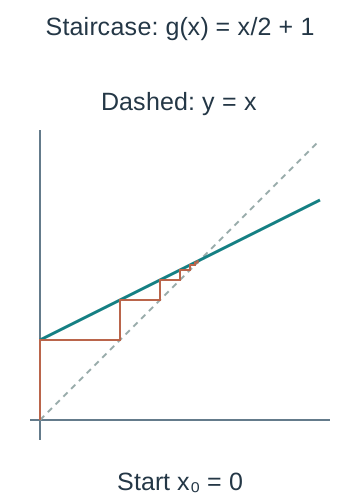
Fixed-point graph — The root of x=g(x) appears where y=g(x) intersects y=x. Start at the chosen x-value on the horizontal axis, move vertically to y=g(x), then horizontally to y=x; the new horizontal coordinate is the next iterate. Repeat this construction rather than draw arrows on unrelated points.
Staircase behaviour — For a suitable increasing g with local slope between zero and one, iterates can approach the fixed point from one side in a staircase pattern. The cubic-root rearrangement has g′(x)=1/[3(x+2)²ᐟ³] near its positive root, a positive magnitude below one. This supports local attraction, with a suitable starting region still needed.
The illustrative linear map g(x)=x/2+1 has fixed point two and positive derivative one half. From x₀=0, the brown vertical-to-map then horizontal-to-diagonal steps approach two from below. Both axes use 80 pixels per unit. This simple geometry example is distinct from the notes numerical cubic-root map, which has analogous positive-slope local staircase behaviour.
Cobweb behaviour — For a decreasing g with local derivative between −1 and zero, iterates can alternate on opposite sides while approaching the fixed point. The illustrative linear iteration g(x)=2−x/2 has fixed point 4/3; from zero it gives 2, 1, 3/2, 5/4,… . It is analytically solvable but useful for seeing the alternating cobweb geometry.
For the illustrative decreasing map g(x)=2−x/2, the fixed point is 4/3 and derivative −1/2. From zero, outputs 2, 1, 3/2, 5/4,… alternate around that value; the brown graphical steps move vertically to g and horizontally to the dashed diagonal. Equal 80-pixel scales preserve the y=x diagonal geometry.
Local derivative criterion — The condition |g′(α)|<1 gives a locally attracting fixed point, one that sufficiently nearby iterates move towards, under the usual smoothness conditions, while |g′(α)|>1 is repelling. This is local information, not a guarantee from every starting value. Equality at one in magnitude is inconclusive and needs more analysis.
Divergent rearrangement — The same cubic equation can be written xₙ₊₁=xₙ³−2. Near its positive root the derivative 3x² is greater than one, so the fixed point is repelling. Starting at 1.5 gives 1.375 then 0.599609375, moving away rather than matching the convergent cube-root rearrangement.
Cycles and boundary cases — The rule xₙ₊₁=1/xₙ from x₀=2 alternates 2 and 1/2 forever. Small finite values or bounded iterates do not establish convergence. Near the fixed point one the derivative is −1, illustrating why the boundary criterion cannot be declared automatically convergent.
Stopping with evidence — Close consecutive iterates suggest stabilisation but should be checked against the original residual and, where required, a rigorous continuous sign bracket for the requested accuracy. Near a rounding plateau an iteration may look unchanged despite insufficient stored precision. Keep guard digits and distinguish a stopping rule from a proof.
Residual versus root error — For f(x)=(x−1)³ at x=1.01, the residual is only 0.000001 but input error is 0.01. A flat graph can have a tiny residual relatively far from a root. Interpret tolerance in the quantity the question specifies rather than assume every small f(x) certifies the same number of decimal places in x.

Newton–Raphson geometry calculation and failure modes

Tangent update — At xₙ, the tangent equation is y=f(xₙ)+f′(xₙ)(x−xₙ). Its x-intercept gives xₙ₊₁=xₙ−f(xₙ)/f′(xₙ), provided the derivative exists and is nonzero. The tangent intercept is the next estimate, not generally the actual curve root after one step.
Derivative and original function — Differentiate the original f accurately before substituting the current estimate. For f=x³−x−2, f′=3x²−1, so the update subtracts (xₙ³−xₙ−2)/(3xₙ²−1). Using f(xₙ) where f′ is needed or reversing the subtraction changes the method.
Worked Newton values — Starting the cubic at x₀=1.5 gives x₁≈1.521739130, x₂≈1.521379806 and x₃≈1.521379707. This is much faster in this example than the earlier fixed-point rearrangement. Speed in a successful example is not a universal guarantee of convergence.
Geometric sequence of tangents — Plot the current point on the curve, draw its tangent to the horizontal axis and take that intercept as the next x-value. Then move vertically back to the curve before forming the next tangent. Connecting two curve estimates with a secant is a different construction and does not explain the Newton derivative formula.
This geometry illustration starts the cubic at x₀=1, where f=−2 and f′=2, giving tangent intercept x₁=2. The dashed vertical returns from that intercept to the curve before another tangent is formed. It uses a different explicitly labelled start from the worked x₀=1.5 table. Horizontal scale is 200 pixels per input unit and vertical scale 35 per output unit; the first tangent intercept is not the actual curve root.
Zero derivative failure — For f=x³−1, starting at x₀=0 gives f′(0)=0 and the update is undefined. A horizontal tangent has no finite x-intercept unless it coincides with the axis, so the tangent picture explains the division failure. Choose a different allowed start or another justified method rather than divide by zero.
Small derivative jump — For the same function at x₀=0.1, the residual is −0.999 and derivative 0.03, producing x₁=33.4. A very shallow tangent can send the estimate far away even though a root lies at one. This jump may be inefficient or leave a valid modelling domain; it does not prove that every later iterate must diverge.
Newton cycle — For f=x³−2x+2, x₀=0 gives x₁=1 and x₂=0, so the process cycles. Both derivatives used are nonzero, yet convergence fails. A valid formula and bounded repeated values alone are not proof of success.
For f=x³−2x+2, the tangent at x=0 takes the estimate to one and the tangent at one takes it back to zero. The brown closed update path includes vertical returns to the curve. Both slopes are nonzero, but the cycle does not approach the actual negative root outside this viewport. Horizontal scale is 200 pixels per input unit and vertical scale 80 per output unit.
Domain escape — For f(x)=ln x starting at x₀=10, the first update is 10−10 ln 10, which is negative. The original function is then undefined over the reals, so the next step is invalid. Check domain restrictions after every update rather than treat all calculator outputs as permitted inputs.
Different roots and starts — A function with several roots can attract different initial estimates to different solutions. A Newton iterate can leave an initial bracket because the method does not automatically preserve its endpoint signs. Verify the requested root interval or physical range and use a bracketed method when a maintained bound is essential.
Precision and certification — Retain sufficient internal precision, report enough iterations to show the required stabilisation and verify the original equation. For a certified decimal result, a final sign bracket can supplement the approximate Newton values. An exactly displayed zero residual after rounding is not proof that the mathematical root is exactly that finite decimal.
Choosing a method — Bisection maintains a continuous sign bracket but can require many steps; fixed-point iteration depends strongly on rearrangement; Newton uses derivatives and can be rapid near a suitable root. Choose with the equation's domain, derivative behaviour, starting information and required error evidence in mind. No method removes the need to interpret its result.

Trapezium rule curvature and numerical bounds

Trapezium approximation — Approximate each small curve section by its joining straight chord and add the trapezia. For equal spacing h=(b−a)/n, ∫ from a to b of f(x) dx is approximately h[y₀+yₙ+2(y₁+…+yₙ₋₁)]/2. There are n strips and n+1 ordinates, the graph heights y₀ through yₙ; the interior heights receive weight two.
Unequal spacing — If adjacent inputs are not equally spaced, sum (xᵢ₊₁−xᵢ)(yᵢ+yᵢ₊₁)/2 for each interval separately. A single common h would be unjustified. Read the actual table rather than infer equal spacing from an unticked illustrative graph.
Worked trapezium table — For f=x²+1 on [0, 1] with h=1/4, the five ordinates are 1, 17/16, 5/4, 25/16, 2. The estimate is (1/8) × [1 + 2 + 2(17/16 + 5/4 + 25/16)] = 43/32 = 1.34375. Keep endpoint and interior weights distinct.
Four strips and five exact ordinates for x²+1 on [0, 1] give trapezium estimate 43/32. The green quadratic lies slightly below its joining chords because it is convex, while its exact integral is 4/3. Horizontal scale is 240 pixels per unit and vertical scale 120; the shaded trapezia extend to the y=0 axis, including the constant-one contribution.
Comparison with exact integration — The exact integral of x²+1 from zero to one is 4/3, so this trapezium estimate is higher by 1/96. The exact value is used here to review the method; in another problem no simple antiderivative may be available. A numerical method remains useful without an exact comparison.
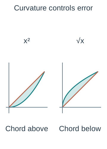
Convex overestimate — For a curve bending upward throughout an interval, its joining chords lie above it, so the trapezium signed-integral estimate is above the true integral. The example x²+1 has f″=2>0 and therefore an overestimate. Use the curve's actual bending rather than infer error direction just from increasing values.
Both panels show the unit interval with equal 120-pixel coordinate scales. The chord of the convex x² graph lies above it, giving an overestimate; the chord of concave √x lies below it, giving an underestimate. These one-chord shape illustrations clarify error direction independently of increasing/decreasing behaviour.
Concave underestimate — For a curve bending downward, chords lie below the graph and the trapezium estimate is below the integral. The function √(2x+1) on [0, 1] is a suitable example. If bending changes within the interval, one overall over/under conclusion may not follow without splitting or further reasoning.
Monotone rectangle bounds — For a positive increasing function with equal-width strips, left-endpoint rectangles give a lower bound and right-endpoint rectangles an upper bound. For x²+1 with four strips, the bounds are 39/32 and 47/32. The exact integral and trapezium estimate lie between these in the example; distinguish rigorous bounds from an approximate middle estimate.
Decreasing and mixed behaviour — For a positive decreasing function, left rectangles are the upper bound and right rectangles lower. A function changing monotonicity needs separate treatment or another valid bound. A curve below the axis still has a signed integral, so physical-area statements also need the sign interpretation from the integration chapter.
Refining the spacing — Reducing strip width generally improves a smooth trapezium approximation and the sums converge for a suitable continuous integrand. Compare successive estimates without declaring their difference an automatic certified error bound. The observed agreement can hide cancellation or unresolved curvature unless a justified bound is available.
Tables and uncertainty — An estimate from observed ordinates inherits rounding or measurement uncertainty as well as the straight-chord approximation between them. Extra arithmetic digits do not create more accurate source measurements. State whether the values are fictional illustrations, exact function evaluations or measured data.
Area versus rate accumulation — Numerical integration may estimate area, volume from a flow rate or displacement from velocity. Multiply units consistently and distinguish signed displacement from travelled distance if velocity changes sign. If only sparse values are available, an assumed interpolation between them is part of the model rather than a directly observed continuous curve.

Numerical models reporting and checking

Fictional flow example — A fictional flow-rate table at times 0, 2, 4, 6 minutes gives rates 3, 5, 4, 2 litres per minute. Three trapezia of width two give total volume (2/2) × [3 + 2 + 2(5 + 4)] = 23 litres. The calculation assumes straight-line interpolation of rates and does not claim these are actual measurements.
The dark ordinates are fictional rates 3, 5, 4, 2 L/min at 0, 2, 4, 6 minutes. Assuming straight-line change between samples gives three trapezia and total 23 litres. Horizontal scale is 40 pixels per minute and vertical scale 40 pixels per L/min. The graph depicts the interpolation assumption, not an actual measured continuous flow.
Nonlinear height equation — A fictional rising-point model uses H(t)=t+e^−t metres when t is its numerical time in seconds, with the coefficients interpreted in those units. To find height 2 m, solve f(t)=t+e^−t−2=0. On [1, 2] the endpoint signs differ and f′=1−e^−t>0, giving a unique root there.
Height Newton calculation — Starting at t₀=1.5, the tangent updates give approximately 1.856391542, 1.841426557, 1.841405660 seconds. Check every value stays in the permitted model interval and verify a final bracket if a certified rounded time is required. Starting at zero would instead have a zero derivative and fail.
Choosing meaningful precision — A time answer needs seconds and an accuracy justified by the question or model, not every calculator digit. Distinguish decimal places from significant figures and a residual measured in height units from an error in seconds. State the interval and method used, together with the evidence supporting the reported accuracy.
Physical and mathematical checks — Substitute the result into the original model, verify the physical range and distinguish one solution from all possible solutions. A maintained sign bracket or monotonicity argument supports existence or uniqueness only where its conditions hold. Do not infer that a numerical algorithm has certified real-world assumptions.
Limitations and refinement — A flow interpolation ignores unobserved variation between sample times; a fitted height model may fail outside the interval where its behaviour is plausible. Propose more frequent data or a better-supported model for a specific identified limitation. More iterations cannot correct an unsuitable equation or inaccurate source data.
Reproducible working — Record the equation, derivative or rearrangement, initial values, iteration outputs, stopping criterion, bounds and units. Retain enough guard digits for another learner to reproduce the result, while rounding the final answer appropriately. A bare calculator root without interval or method evidence does not demonstrate the numerical reasoning.

Test yourself

50 questions · Random sets of 10. These quick checks support revision; practise longer explanations and justified judgements too.