Sample space — A sample space lists the possible outcomes under a defined experiment. For two ordered coin tosses, {HH,HT,TH,TT} has four outcomes; order distinguishes HT from TH. Whether these outcomes are equally likely is an additional model assumption, not a consequence of listing them.
Events as sets — An event is a set of outcomes, such as exactly one head {HT,TH}. The probability of an event is the total probability assigned to its outcomes. Use P(A)=number of favourable outcomes/number of possible outcomes only when the elementary outcomes being counted are equally likely.
Probability bounds — Every probability lies between zero and one inclusive. The certain event has probability one and the impossible event has probability zero. In finite equally likely models a nonempty event has positive probability; later continuous models can assign probability zero to a single possible exact value without making the outcome logically impossible.
Complement — The complement A′ contains all outcomes in the sample space that are not in A, and P(A′)=1−P(A). An outcome belongs to exactly one of A and A′. Define the full reference population before taking a complement; not having attribute A is not necessarily the same as having a separately named attribute B.
Intersection and union — A∩B means both events occur; A∪B means at least one occurs, including both. Everyday use of either can be ambiguous, so translate the intended event explicitly. A person in both clubs belongs to the union and must be counted once, not excluded or counted twice.
Addition rule — P(A∪B)=P(A)+P(B)−P(A∩B). Subtract the overlap once because it was included in each of the first two terms. If P(A)=0.6, P(B)=0.5 and overlap is 0.3, the union is 0.8 and neither has probability 0.2.
Mutually exclusive events — Events are mutually exclusive when A∩B is empty, so they cannot occur on the same trial. Their intersection probability is zero and their union probability is the sum. Describing clubs as different does not establish exclusivity: an individual might belong to both.
Exhaustive events — A collection is exhaustive if its union covers the entire sample space. Exhaustive does not mean mutually exclusive: two overlapping events can still cover everyone. A partition is both exhaustive and pairwise mutually exclusive, so it provides nonoverlapping cases for totals.
Consistency of assigned probabilities — An overlap cannot exceed either event probability. Also P(A∩B) must be at least max(0,P(A)+P(B)−1). For probabilities 0.7 and 0.6, an overlap below 0.3 would imply a union above one and is therefore impossible.
Set transformations — Not both is the complement of A∩B and equals A′∪B′; neither is A′∩B′, the complement of A∪B. These are different events. With overlap 0.3 and union 0.8, not both has probability 0.7 while neither has probability 0.2.
Venn diagrams two-way tables and event accounting
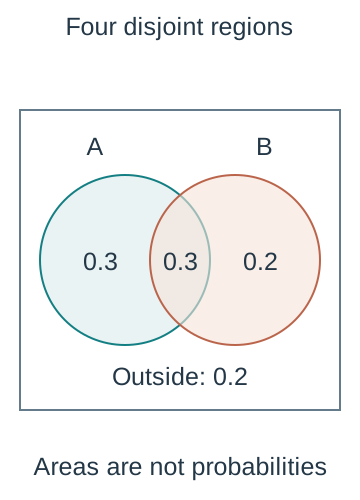
Venn regions — For two events, separate A only, B only, both and neither. If P(A)=0.6, P(B)=0.5 and both is 0.3, the four regions are 0.3,0.2,0.3,0.2 respectively. Check their total is one before answering a question that combines regions.The schematic labels the four disjoint probabilities A only 0.3, both 0.3, B only 0.2 and neither 0.2. Circle areas are deliberately not proportional to probabilities. Summing the three inside regions gives union 0.8; exactly one sums only the two outer regions to 0.5.
Exactly one — Exactly one of A and B includes the two exclusive regions and excludes the overlap. It has probability P(A)+P(B)−2P(A∩B). In the worked example it is 0.5, distinct from the union 0.8 and from the intersection 0.3.
Three-event diagrams — Start a three-circle diagram with the triple intersection, then fill each pair-only region by subtracting the triple from the stated inclusive pair total. Finally calculate single-only regions and the outside. A statement such as twenty attend A and B normally includes any who also attend C unless the wording says only.
Worked three-event count — In a fictional population of 100, suppose totals are A=45,B=40,C=30, with inclusive pair counts AB=15,AC=12,BC=10 and ABC=5. Pair-only counts are 10,7,5; single-only counts are 23,20,13. The union is 83 and neither any of the three is 17; all eight regions together total 100.
Two-way table — A two-way table cross-classifies the same observational units by two categorical variables. Every unit must occupy exactly one interior cell if categories are exhaustive and mutually exclusive. Row and column margins are totals, not additional observations to add to the grand total.
Worked table — A fictional sample of 200 has A∩B=48, A∩B′=32, A′∩B=72 and A′∩B′=48. Row totals for A,A′ are 80,120; column totals for B,B′ are 120,80. Thus P(A)=0.4, P(B)=0.6 and P(A∩B)=0.24. Counts must all describe the same sample.
Relative frequencies — Dividing table cells by the grand total estimates unconditional probabilities for a randomly selected record. Dividing within a row or column instead answers a conditional question. Empirical means based on observations. Empirical proportions describe the observed sample; applying them to a wider population requires assumptions about the collection process and representativeness.
Missing categories and overlaps — If some observations are unclassified, unknown is not automatically the complement of a known category. Likewise overlapping response categories cannot be treated as a partition without restructuring the table. Explain the actual denominator and classification rule rather than fill a missing table cell by an unjustified complement.
Checking representations — Translate a probability statement into a region or table cell before calculating. Verify that margins, region sums and the grand total agree, and check whether the requested selection is from everyone or an identified subgroup. A correct count divided by the wrong total answers a different event.
Conditional probability restricted spaces and reversed conditions
Conditional definition — For P(B)>0, P(A given B)=P(A∩B)/P(B). The condition B restricts the reference space to outcomes where B occurs. The numerator must satisfy both A and B; the denominator includes all permitted outcomes in B, whether or not A occurs.
Conditional table calculation — In the fictional 200-record table, P(A given B)=48/120=0.4, whereas P(B given A)=48/80=0.6. They use the same overlap but different restricted populations. Swapping the words after given changes the question and generally changes the probability.The fictional two-way table contains four interior counts and their row/column totals. Given B restricts the denominator to 120; given A restricts it to 80. The common numerator 48 therefore gives conditional probabilities 0.4 and 0.6 respectively. Margins summarise existing units, not additional observations.
Zero-probability conditions — The elementary conditional formula cannot be used when P(B)=0 because it would divide by zero. Do not invent a conditional probability by cancelling or assigning zero automatically. In this course's finite models, a stated condition must have positive probability for this formula to be meaningful.
Conditional complements — Within the same positive-probability condition B, P(A′ given B)=1−P(A given B). The complement changes the event being assessed while retaining B as the reference space. Replacing the condition by B′ is a different operation and is not obtained by the same subtraction.
Conditional multiplication — Rearranging the definition gives P(A∩B)=P(B)P(A given B). Equally, when P(A)>0, use P(A)P(B given A). Choose the order that matches known information; neither product assumes independence because the second factor is explicitly conditional.
Total probability by cases — If B and B′ form a partition with relevant conditions defined, P(A)=P(B)P(A given B)+P(B′)P(A given B′). The paths are mutually exclusive ways A can occur. Extend to more than two exhaustive disjoint cases by summing all corresponding products.
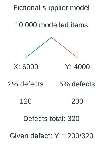
Reversing a condition by accounting — Suppose fictional suppliers X and Y provide 60% and 40% of items, with defect rates 2% and 5%. The defect probability is 0.6×0.02+0.4×0.05=0.032. Given an item is defective, the probability it came from Y is (0.4×0.05)/0.032=0.625. The numerator and denominator must both refer to defective items.
Natural-frequency explanation — Imagine 10000 items under that model: 6000 from X produce an expected 120 defects and 4000 from Y an expected 200. Of 320 expected defects, 200 are from Y, giving the same 0.625. These are model-expected counts for explanation, not actual measured factory results or a guarantee for a sample of 10000.Under the fictional mixture model, expected source counts 6000 and 4000 in a reference population of 10000 produce expected defect counts 120 and 200. Conditioning on the 320 total defects gives probability 200/320=0.625 of source Y. These are model-expected counts and not observed factory measurements.
Base rates and reversed questions — A high P(positive result given condition) does not itself give a high P(condition given positive result). The underlying prevalence (how common the condition is) and false-positive rate (how often the test is positive without the condition) affect the latter denominator. Use a labelled fictional screening or classification model to practise the arithmetic, not as personal medical or real-world decision advice.
Conditional union — Inside a fixed condition C of positive probability, P(A∪B given C)=P(A given C)+P(B given C)−P(A∩B given C). All terms share the same restricted reference population. Mixing an unconditional term with conditional terms generally breaks the accounting.
Tree diagrams successive selections and replacement
Tree structure — The first branches give initial-event probabilities; later branches give probabilities conditional on the path already followed. Branch probabilities leaving any reachable node sum to one. Label the outcomes and whether objects are replaced before assigning later-stage probabilities.
Multiplying a path — Multiply probabilities along one path to obtain the joint probability of its successive outcomes. The multiplication is valid because each later branch is conditional on the earlier stages. It does not require the branch events to be independent.
Adding complete paths — Sum probabilities of distinct complete paths corresponding to the requested event. In a correctly constructed tree these paths are mutually exclusive descriptions, so they can be added without overlap subtraction. Check that the selected paths are exhaustive for the event, especially for at least one or exactly one.
Without replacement example — A bag has three red and two blue counters. Drawing two without replacement gives P(RR)=(3/5)(2/4)=3/10 and P(BB)=(2/5)(1/4)=1/10. The second denominator is four because one object has been removed; the available colour count depends on the first outcome.For three red and two blue counters sampled twice without replacement, the first branches are 3/5 and 2/5. Conditional second branches update the remaining colour counts over denominator four. Complete RR,RB,BR,BB paths have probabilities 0.3,0.3,0.3,0.1. The first and third second-stage probabilities differ because the earlier outcomes differ.
Different colours — For that bag without replacement, P(RB)=(3/5)(2/4)=3/10 and P(BR)=(2/5)(3/4)=3/10. Different colours therefore has probability 3/5, not just the probability of one ordering. Both ordered paths must be counted unless the sample-space construction already combines them.
With replacement example — If a counter is returned and the bag mixed before the second draw, the colour proportions are restored. Under the random-draw model, P(RR)=(3/5)²=9/25 and P(different colours)=2(3/5)(2/5)=12/25. Replacement supports unchanged stage probabilities; independent random selection remains a modelling assumption about the procedure.
At least one by complement — In the without-replacement bag example, at least one red is the complement of BB and has probability 9/10. With replacement it is 1−(2/5)²=21/25. Check the complement model rather than use a memorised formula without the replacement distinction.
Inferring an earlier stage — Given exactly one red among the two without-replacement draws, P(first red)=P(RB)/P(exactly one red)=(3/10)/(3/5)=1/2. The condition restricts the tree to the two surviving paths RB and BR; it does not leave the original first-draw probability unchanged.
Multiple stages — For three or more selections without replacement, update both remaining counts and denominators after each specified outcome. Under replacement, repeated trials may share a constant success probability, but count the number of distinct ordered paths when an event permits several arrangements. Later binomial methods organise this only when their assumptions hold.
Independence mutual exclusivity and model criticism
Definition of independence — Events A and B are independent when P(A∩B)=P(A)P(B). If P(B)>0, this is equivalent to P(A given B)=P(A); observing B does not change the probability of A in the model. Independence concerns probabilities, not whether event names or physical objects look different.
Worked independent table — The fictional table has P(A∩B)=0.24 and P(A)P(B)=0.4×0.6=0.24, so its empirical relative-frequency distribution satisfies the product relation exactly. This arithmetic checks the table; treating a future population process as independent needs evidence beyond matching one small observed table.
Worked dependence — If P(A)=0.6,P(B)=0.5 and P(A∩B)=0.3, the product relation also holds. Changing only the overlap to 0.4 would make the events dependent: P(A given B)=0.8 differs from 0.6. A Venn diagram can show either case, so circles overlapping does not by itself establish dependence.
Independent versus exclusive — Mutually exclusive positive-probability events have intersection zero but product greater than zero, so they cannot be independent. If one event has probability zero, the product criterion needs separate interpretation; do not claim the two concepts are universally incompatible without the positive-probability qualification.
Complements preserve independence — If A and B are independent, A′ and B are independent because P(A′∩B)=P(B)−P(A∩B)=(1−P(A))P(B). The same reasoning applies to other complements. This follows from the model relation rather than from an assumption that all complements are independent.
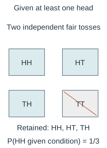
Conditioning can change independence — Two independent fair coin tosses have independent first-head and second-head events. Given at least one head, the restricted outcomes are HH,HT,TH, so each head event has conditional probability 2/3 but both has conditional probability 1/3, not 4/9. Independence in a full space need not survive restriction to a subgroup.The four original ordered outcomes of two independent fair tosses each have probability one quarter. Conditioning on at least one head excludes TT and leaves three equally likely outcomes. HH then has conditional probability one third, while each individual head event has conditional probability two thirds; their product four ninths is different, so independence does not remain.
Pairwise and multiple independence — For three events, checking each pair alone does not generally justify multiplying all three marginal probabilities, the individual event probabilities before any further conditioning. For two independent fair tosses, let A be first head, B second head and C matching results. Each pair has intersection probability 1/4 with marginals 1/2, yet P(A∩B∩C)=1/4 differs from 1/8. This counterexample clarifies why a model must support the full multiplication it uses.
Empirical evidence and assumptions — A tree or Venn diagram represents the assumptions supplied to it; drawing one does not establish fairness, equal likelihood or independent trials. Repeated weather observations may be seasonally related, and sampling without replacement changes later probabilities. Identify which assumption is threatened and how that affects the calculation.
Continuous geometric probability — In a uniform selection model over a finite interval or region, probability is an appropriate length or area fraction. For a point chosen uniformly from [0,10], P(2≤X≤5)=3/10, while a single exact value has probability zero. Equal length intervals have equal probabilities only under the stated uniform model; formal density-function formulae are not required here.A uniformly selected point on the interval from zero to ten lies between two and five with probability length three divided by length ten. The horizontal scale is 28 pixels per unit. Endpoint inclusion does not change this continuous probability because exact endpoints have probability zero.
Evaluating a result — Check probability bounds, event wording, denominator, disjointness of added cases and the assumptions behind multiplied factors. State whether a number is exact within a supplied model or an empirical estimate. Explain how a specific alternative selection procedure or dependence could alter the conclusion rather than merely write that real life is complicated.
Test yourself
50 questions · Random sets of 10. These quick checks support revision; practise longer explanations and justified judgements too.
 Mr Kidman's Classroom