Population and sampling unit — A population is the complete collection relevant to an investigation, and a sampling unit is one member that could be selected. State the population precisely, including place and time: all pupils enrolled at a school this term differs from all pupils who attend on one particular day. The population need not consist of people.
Sample and census — A sample observes a subset; a census attempts to observe every population unit. A census avoids sampling variation for its defined population but can still suffer missing responses, measurement error or misleading questions. It may be expensive, slow or destructive, while a smaller carefully selected sample can answer a narrower question efficiently.
Frame and coverage — A sampling frame lists the eligible units from which selection occurs. Missing pupils, duplicate records or an obsolete list change who can be selected. Check frame coverage before describing a selection as representative; a random choice from an incomplete frame does not repair the excluded group's absence.
Simple random sampling — For a simple random sample of size n without replacement, every possible n-member subset has the same selection probability. Number the eligible frame, use a suitable random generator and reject repeats and out-of-range values until n distinct units are selected. Marginal here means the overall chance of selecting one named unit without specifying its companions in the sample. Equal marginal selection chances alone do not prove all possible subsets are equally likely.
Randomness and realised samples — Random selection reduces systematic selection bias but does not guarantee any particular sample perfectly matches the population. Different legitimate samples give different summaries through sampling variation. A larger random sample generally reduces that variation, but increasing the size of a biased convenience sample does not remove its selection mechanism.
Systematic method — When N=kn, choose a random start from 1 to k and take every kth entry. For 240 entries and a sample of 24, k=10; a start of 7 selects 7,17,…,237. A known periodic pattern in the list could align with the interval and distort the selection, so examine ordering as well as convenience.
Stratified method — Divide the population into mutually exclusive strata covering the population, nonoverlapping groups such as school year groups, then select randomly within each. A proportional allocation uses n_h=nN_h/N. With strata of 120,80,40 and sample 24, select 12,8,4. If allocations are nonintegers, use a justified rounding arrangement preserving the total; disproportionate allocations require care when forming a population summary.Bars show fictional population strata 120,80,40 on the same horizontal size scale, with proportional sample allocations 12,8,4 from a total sample of 24. Selection must still be random within each stratum; the bars alone do not implement that selection.
Quota method — Set target numbers for categories, then allow selection of accessible units within them rather than random selection from complete category frames. Matching quotas can secure some category balance cheaply but still leave interviewer or availability bias within each category. Quota sampling is not stratified random sampling simply because both use groups.
Opportunity method — Select units readily available at the time and place of collection. Asking the first willing people near a sports hall is quick but may miss people who use other facilities or attend at different times. Explain the actual excluded group and its plausible relevance rather than write only that the method is biased.
Nonresponse and replacement — Selected people who do not respond can differ systematically from respondents. Report response rates and follow-up arrangements; quietly replacing every nonrespondent with a nearby volunteer changes the selection procedure. Random initial selection does not guarantee unbiased final responses.
Question and measurement design — Use a stated period, nonoverlapping response categories and neutral wording. Asking how often someone exercises without defining an activity or time window produces incomparable answers. A pilot can expose ambiguity, missing categories and inconsistent measuring procedures before the main collection.
Designing an investigation — Connect the research question, population, frame, variable definitions, selection method and practical constraints. Justify compromises and explain the limits of generalising beyond the observed setting. Statistical arithmetic cannot turn an unrepresentative or badly measured sample into reliable evidence for a broader claim.
Data types frequency tables and graphical presentation
Types of variable — Qualitative variables describe categories; quantitative variables are numerical quantities. Quantitative discrete variables take separated possible values, often counts, while continuous variables can take any value over an interval in a model. A numerical category code does not make a nominal category, one whose labels have no numerical size or ranking, into a measured quantity.
Recorded versus underlying values — A continuous measurement rounded to one decimal place appears on a discrete recording grid, but the underlying variable may remain continuous. An observed value 12.4 rounded to the nearest 0.1 represents 12.35≤x<12.45 under the stated convention. Counts of events are discrete for a different reason: fractional event counts are not possible.
Class boundaries — State intervals so each value belongs to exactly one class. For measurements rounded to whole units, a recorded class 10–19 can correspond to underlying boundaries 9.5 and 19.5. Use the question's measurement convention rather than automatically shifting every written interval by one half.
Frequency and relative frequency — Frequency is the number in a class; relative frequency divides by the relevant total. Check that exhaustive nonoverlapping class frequencies sum to the sample size. Missing observations may make the denominator smaller than the number of records originally selected, so state which observations are included.
Histograms and density — A histogram represents frequency by rectangle area, not height alone. Frequency density is frequency divided by class width. For widths 5,5,10 and frequencies 10,15,20, densities are 2,3,2; the final wider class has the most observations despite not being tallest. Label both the measurement axis and density axis.For fictional classes [0,5),[5,10),[10,20), frequencies 10,15,20 give densities 2,3,2. Horizontal scale is 12 pixels per measurement unit and vertical scale 60 pixels per density unit. The last bar is twice as wide as either earlier one; its area represents the greatest count despite its lower height.
Recovering frequency from a graph — With a labelled density scale, multiply bar height by class width. If the vertical scale is omitted, a known class frequency can establish an area-to-frequency factor used for other bars. Width must be measured in the horizontal variable's units, not by the number of printed class labels.
Frequency polygons — Plot each class midpoint against its frequency and join successive points with straight segments. A polygon summarises grouped data and is not the same construction as a cumulative curve. Make frequencies, class widths and any comparison basis clear so unequal grouping or different totals do not invite a misleading visual comparison.
Cumulative frequency — The cumulative count at an upper class boundary totals observations below that boundary, following the stated endpoint convention. Begin with zero at the lowest boundary and accumulate class frequencies. A cumulative curve should not decrease; its final value should agree with the number of included observations.
Percentiles from cumulative data — For a grouped sample of n, locate the cumulative count pn for the pth fraction, then interpolate within the containing class if required. With class 10≤x<20 containing 30 observations, cumulative count 20 below it and n=100, the lower quartile estimate is 10+((25−20)/30)×10=35/3. This assumes observations are distributed uniformly within that class.A partial fictional cumulative curve has count 20 at upper boundary 10 and count 50 at upper boundary 20. With sample size 100, the lower quartile is estimated at cumulative count 25. The joining segment assumes uniform spread within the class. Horizontal scale is 12 pixels per measurement unit and vertical scale 3 pixels per count; the remainder of the distribution beyond 20 is not drawn.
Box plots — A box plot displays a median, quartiles and whiskers; separate outliers may be plotted according to a stated rule. Check whether whiskers end at extreme observations or at the most extreme nonoutliers. It summarises location and spread but conceals sample detail and does not reveal multimodality, several distinct peaks in a distribution, by itself.
Comparing distributions — Compare a suitable location measure and spread measure in context, with values and units where available. A higher median journey time and a larger interquartile range (IQR) mean a longer typical central journey and more variable middle-half times; neither alone proves every journey in one group exceeds every journey in the other.
Selecting and critiquing graphs — Use a graph appropriate to the variable and question. Check denominators, missing observations, horizontal widths, axis breaks and scales before drawing a comparison. A chart can accurately reproduce counts while a selective time window or omitted category still leads to an unsupported conclusion.
Location spread coding and grouped estimates
Arithmetic mean — For n values, x̄=Σx/n; with frequencies, x̄=Σfx/Σf. Include repeated observations through their frequencies and distinguish a mean of all observations from an unweighted mean of group means. Combining groups requires their sizes as weights unless the group sizes are equal.
Median convention — Order the raw observations. For odd n use the central observation and for even n average the two central observations. Quartile conventions for finite ungrouped samples can differ between instructions and calculator settings; use the question's stated convention consistently rather than claim every method returns the same quartiles.
Mode and modal class — The mode is the most frequent recorded value and may not be unique. A modal class summarises grouped observations, but unequal-width histogram height identifies density, not necessarily the class with largest frequency. Read whether the question asks for modal class by frequency or greatest concentration per unit width.
Range and interquartile range — Range is maximum minus minimum and uses the extreme observations. IQR=Q₃−Q₁ describes the spread of the middle half and is less sensitive to extremes. An interpercentile range similarly subtracts specified percentiles, such as P₉₀−P₁₀; retain the measurement units.
Variance from deviations — For descriptive variance with denominator n, variance=(Σ(x−x̄)²)/n. Squared deviations prevent positive and negative differences cancelling; its units are squared measurement units. Standard deviation is the nonnegative square root and returns to the original units.
Summary formula — Define Sxx=Σx²−(Σx)²/n. Then descriptive variance=Sxx/n and standard deviation=√(Sxx/n). Keep Σx² distinct from (Σx)². With values 2,4,4,6, Σx=16 and Σx²=72, giving mean 4, variance 2 and standard deviation √2.Fictional raw observations 2,4,4,6 have mean 4. The repeated four is stacked vertically for visibility, not assigned a different measurement. Signed deviations −2,0,0,2 have squared total 8, giving descriptive variance 2 when divided by four observations.
Alternative denominator — Some software reports a sample standard deviation √(Sxx/(n−1)) rather than the descriptive √(Sxx/n). The Edexcel guidance accepts the sample-denominator form in this context, but the two numbers are not identical. Identify the formula or calculator output actually used, especially when comparing reported results.
Frequency summary formula — For frequency data use n=Σf, total Σfx and square total Σfx². Thus variance=(Σfx²/Σf)−x̄² for the descriptive denominator. Squaring fx before summing is incorrect: x² is weighted by frequency, not by frequency squared.
Grouped mean estimate — Replace each value in a class by its midpoint and compute Σfm/Σf. For classes [0,5),[5,10),[10,20) with frequencies 10,15,20, the estimated total is 10×2.5+15×7.5+20×15=437.5 and mean 175/18≈9.722. This is an estimate because the actual within-class values are unknown.
Grouped spread estimate — Use the same midpoint approximation in the square-total formula to estimate variance or standard deviation. For those classes, Σfm²=5406.25, giving descriptive variance 2075/81 and standard deviation 5√83/9≈5.061. The method treats all observations in a class as its midpoint, so the grouping loses information about true spread.
Combining summary data — For separate nonoverlapping groups, add their counts, totals and square totals before recalculating a combined mean and variance. Do not average two standard deviations to obtain a combined standard deviation: differences between group means also contribute to the combined spread.
Linear coding — Coding rescales or shifts data to make calculations easier while preserving a known way back to the original measurements. If y=(x−a)/b with nonzero b, then x=a+by. Means transform as x̄=a+bȳ, standard deviations as s_x=|b|s_y and variances as b² times the coded variance. Adding a constant changes location but not spread; multiplying by a negative value reverses order without making standard deviation negative.
Coding example — For y=(x−10)/2 with ȳ=3 and descriptive variance of y equal to 4, x̄=16, variance of x is 16 and standard deviation of x is 4. Calculate these transformations before rounding. The shift ten contributes to the mean but not to variance.
Stable calculation — Use stored calculator values or sufficient guard digits. Rounded means substituted into a difference-of-large-numbers formula can give a misleading variance, even a small negative result. A genuine variance cannot be negative; inspect totals, units, rounding and entered frequency lists rather than take a square root of its absolute value.
Outliers cleaning and honest statistical conclusions
Specified outlier rules — Use the outlier definition supplied in the question. For the rule below Q₁−1.5IQR or above Q₃+1.5IQR, observations exactly on the bounds are not outside them. Another task may specify a mean/standard-deviation rule, which is a different criterion rather than a universal replacement.
Outlier calculation — If Q₁=12 and Q₃=20, IQR=8 and the 1.5IQR fences are 0 and 32. Under a strict outside-fences rule, 33 is an outlier while 32 is not. An outlier classification describes the chosen distribution rule; it does not establish that the observation is an error.With fictional quartiles 12 and 20 and the supplied strict 1.5IQR outside-fence rule, fences are 0 and 32. The value 33 lies outside the upper fence while 32 does not. Horizontal scale is 8 pixels per unit. This is a fence illustration, not a full box plot: no median or whisker observations are supplied.
Investigating unusual values — Compare an unusual value with its source, units, date, duplicate records and plausible context. A very windy day could be a genuine extreme event. Remove or correct a confirmed error with a recorded reason; show or discuss how retaining a plausible extreme affects a summary instead of deleting it to obtain a preferred result.
Missing observations — An unavailable value is not a measured zero. Restrict a two-variable analysis to correctly paired observations where the required values are available, report the resulting sample size and consider whether missingness depends on weather, location or measurement conditions. Different summaries can otherwise refer to different subsets without anyone noticing.
Cleaning and reproducibility — Keep the original records, document exclusions and conversions and create a separate prepared analysis. Treat trace amounts according to an explicit stated convention and assess sensitivity where relevant. Reproducible cleaning makes another person able to understand the denominator and recover the analysis decisions.
Precision and uncertainty — Distinguish sampling variation, measurement rounding, missingness, grouping and model assumptions. More calculator digits cannot correct an unrepresentative sample or restore values lost by grouping. Qualify the conclusion at the level supported by the actual data and collection procedure.
Scatter diagrams regression and association
Paired observations — A scatter diagram plots paired numerical measurements from the same units. Keep both measurements from each date or person together; independently sorting the two columns invents new pairs and changes the association. Label variables and units on the appropriate axes.
Direction form and strength — Describe whether the association is positive, negative or absent, whether it is approximately linear or curved and how closely points follow the pattern. A strong curved relationship may have little linear correlation. A single influential point or two mixed groups can change the apparent whole-sample pattern.Eight invented paired observations illustrate a positive approximately linear association with scatter. The axes identify explanatory and response roles but no numerical dataset or calibrated units are asserted. No causation or exact fitted coefficients are implied by the schematic.
Explanatory and response variables — Choose the explanatory variable x and response y according to the investigation. A fitted regression of y on x predicts y for a specified x and is not generally reversible to predict x by algebraically rearranging the same fit. Both variables can have uncertainty even when one is used for explanation.
Interpreting a supplied line — For a fictional supplied model y=12+0.8x, predicted y increases by 0.8 units for each extra unit of x. The intercept is the predicted y at x=0, which may lack practical meaning outside the observed range. Statistical calculations to obtain regression coefficients are excluded from this specification's regression-line requirement; interpret and use the supplied or technology output appropriately.
Interpolation and extrapolation — Predicting within the observed explanatory range is interpolation; predicting outside it is extrapolation. Even an interpolated estimate can be unreliable if scatter is large or the chosen model is unsuitable. A line fitted to temperatures 8–18°C does not gain evidence for 35°C simply because its formula gives a numerical answer.
Residuals and limitations — A residual is observed y minus the fitted y for the same explanatory input. It records vertical discrepancy, not proof of measurement error. Curved residual patterns suggest an unsuitable straight-line form; an unusual point may warrant investigation rather than automatic deletion.
Correlation coefficient — The product moment correlation coefficient r measures linear association and lies between −1 and 1. Its sign gives direction and its magnitude the closeness of the linear association. A value near zero does not exclude a curved association. Computing r with technology is distinct from the later significance test of a population correlation.
Causation and confounding — Association alone does not establish that changing x causes y to change. A third factor, such as season, may affect both measurements. Comparing pooled locations or months can conceal within-group patterns, so inspect meaningful subgroups before attributing a single explanation to the whole cloud of points.
Linearising models — For y=Aeᵏˣ with y>0 and A>0, ln y=ln A+kx. A straight line on axes x and ln y therefore has gradient k and intercept ln A, requiring exponentiation to recover A. For y=Axⁿ with positive x,y, logarithmic axes give ln y=ln A+n ln x. State transformed variables and domains; a fit in transformed coordinates does not prove the original model is true.
Contextual comparison — Interpret slope, scatter, plausible range, subgroup structure and source limitations together. A strong relationship over selected summer days at one station may not transfer to another place or season. Explain the specific assumption needing evidence rather than merely labelling every prediction unreliable.
The official weather large data set and technology investigations
Weather context — Pearson's large data set uses Met Office weather observations for May–October in 1987 and 2015. Its UK stations are Camborne, Heathrow, Hurn, Leeming and Leuchars; overseas stations are Beijing, Jacksonville and Perth. Know the broad setting and investigate the supplied records rather than memorise every row or treat a fabricated worked example as an actual observation.
Periods and scope — May through October includes 184 calendar days in each year. These dates do not provide year-round coverage: neither a summer sample nor two selected years establish a general long-term climate trend on their own. Define whether a population is the workbook's finite days, a particular station-month or a much broader weather process before making an inference.
Temperature rainfall and sunshine — The relevant units are °C for daily mean air temperature, mm for daily rainfall total and hours for sunshine duration. A daily mean temperature is not the day's maximum. Read each header's observation window: the UK temperature/rainfall descriptions use a 09:00-to-09:00 period, while several other daily measurements use midnight-to-midnight, so a matching displayed date need not mean identical time windows.
Wind measurements — Wind speeds and maximum gusts are given in knots, with the workbook using the approximate conversion 1 knot=1.15 mph. Mean speed and the maximum instantaneous gust are different quantities. Beaufort descriptions are ordered categories rather than another measurement in knots. Do not average category labels as if the words were numerical speeds.
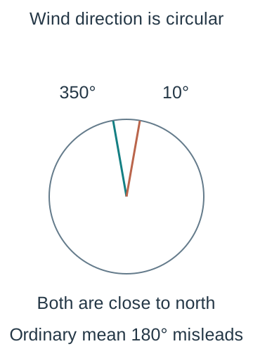
Wind direction interpretation — The UK sheets include numerical wind/gust directions and corresponding compass labels. Meteorological wind direction identifies where wind comes from; it does not directly specify the direction a boat is carried towards. North is close to the 0°/360° boundary, so an ordinary arithmetic average of 350° and 10° incorrectly points south; circular direction requires interpretation.Two rays at bearings 350 degrees and 10 degrees lie on opposite sides of north near the top of the circle. Their ordinary arithmetic average is 180 degrees, which points in the opposite direction. This demonstrates why numerical direction codes need circular interpretation, without imposing an extra circular-statistics calculation method.
Humidity cloud visibility and pressure — Maximum relative humidity is a percentage; cloud cover is recorded in oktas, or eighths; visibility uses decametres; pressure uses hPa. Thus 1200 dam represents 12000 m and 1015 hPa represents 101500 Pa. A cloud value eight indicates full cover, while zero cloud is a legitimate observation rather than missing data.
Variable availability — The overseas sheets contain temperature, rainfall, pressure and mean wind speed, with an accompanying Beaufort category. They do not provide all UK variables such as sunshine or cloud cover. Choose comparisons using variables actually present and check available observations in each subset instead of assuming every sheet has an identical structure.
Trace and missing codes — The workbook identifies tr as rainfall below 0.05 mm and uses unavailable markers such as n/a; its visibility explanation also identifies a dash for missing data. Some direction entries use NA or a corresponding unavailable display. Read the relevant column and supplied notes before converting text: a trace is not an unknown value and an unavailable observation is not a measured zero.
Geography and seasonality — Perth is in the southern hemisphere, so the same calendar months do not represent the same seasonal progression as the UK. Coastal and inland settings, latitude and local conditions can also affect comparisons. Use these as possible contextual explanations to investigate, not as proof that geography alone caused a particular observed difference.
A reproducible workbook sample — For a sample of days at a named station-year, identify the eligible dated rows, assign row identifiers and select without replacement by the stated method. If stratifying by month, allocate and select within each month rather than simply choose the same convenient dates. Preserve the date and all required paired measurements together.
Technology and cleaning — Work on an analysis copy, retain the original and create explicit filters for the required station, year and variables. Count numeric observations and examine text codes before applying mean, spread or chart tools; automatic spreadsheet exclusion of text can silently change the denominator. Record any trace-value convention and inspect whether complete-case selection changes the represented days.
Investigating association — Select meaningful pairs such as temperature and sunshine where both are available, plot them, inspect grouping by month and use technology to explore a correlation and a supplied or computed fitted model. The course encourages practical technology exploration; that activity does not create a requirement to derive regression coefficients by hand. Discuss extrapolation and omitted seasonal influences.
Evidence from real records — An actual investigation should report the chosen sheets, dates, variables, units, sample selection, cleaning decisions and resulting graphs/statistics. Compare distributions using consistent definitions and denominators. The fictional examples elsewhere in these notes practise methods; they are not claims about what the workbook's weather measurements show.
Assessment familiarity — Use the official data set during study to practise sampling, data preparation, visualisation, summary statistics and later inference. Examination extracts needed for calculations are supplied as appropriate; familiarity with context and variable meaning still matters. Quiz recall cannot substitute for carrying out a technology investigation and explaining its limitations.
Test yourself
50 questions · Random sets of 10. These quick checks support revision; practise longer explanations and justified judgements too.
 Mr Kidman's Classroom


![For fictional classes [0,5),[5,10),[10,20), frequencies 10,15,20 give densities 2,3,2. Horizontal scale is 12 pixels per measurement unit and vertical scale 60 pixels per density unit. The last bar is twice as wide as either earlier one; its area represents the greatest count despite its lower height.](/assets/images/ks5/mathematics/data-unequal-histogram.svg)