Population claim — A population parameter is a number describing the population model. A hypothesis is a claim about such a parameter, such as success probability p, normal mean μ or population correlation ρ. The observed sample count, sample mean and sample correlation are evidence about those parameters, not interchangeable names for them. Define the population and parameter in context before testing.
Null and alternative — H₀ specifies a reference parameter value; H₁ states the direction or difference for which evidence is sought. For a claimed success probability 0.4, use H₀:p=0.4 and an appropriate H₁ such as p>0.4. Do not write the null as the observed sample proportion equalling the proposed probability.
One-sided alternatives — An increase question leads to H₁:p>p₀ or μ>μ₀; a decrease leads to the corresponding less-than claim. The tail must follow the research question set before inspecting the sample. Choosing whichever direction looks more impressive after observing the data changes the intended procedure and its error rate.
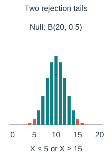
Two-sided alternatives — A change in either direction is represented by H₁:p≠p₀ or μ≠μ₀. Extreme evidence can then arise on both sides of the null-model centre. Allocate the stated significance level across tails as required; comparing each tail to the full two-sided level would generally allow too many rejections.
Test statistic — A test statistic is the sample quantity used for the decision, together with its distribution under H₀. A binomial test may use success count X, a normal mean test uses X̄ or a standardised Z and a correlation test uses sample r. State the null-model distribution before calculating a tail probability.
Significance level — The significance level α controls the probability of rejecting H₀ when its specified model is true. A 5% level does not mean the null hypothesis has probability 5% or that a nonrejected claim is 95% certain. Its error interpretation assumes the sampling procedure and model conditions used by the test.
Critical region — The critical or rejection region contains statistic values leading to rejection of H₀. Its boundary is a critical value, with the inclusive inequality explicitly stated for discrete counts. Values outside it are sometimes called an acceptance region; being there does not prove H₀ true.
P-value — A p-value measures, under the null model, the probability of evidence at least as extreme as the observed result according to the specified alternative and testing procedure. It is not the probability that H₀ is true and not the probability that the observed exact outcome occurs alone. Calculate the appropriate tail or two-tail evidence.
Decision rule — Compare the appropriate p-value with α, or compare the observed statistic with the pre-established critical region. State the convention at an exact boundary, normally reject for p-value≤α. Keep adequate internal precision so premature rounding does not reverse a close decision.
Contextual conclusion — Rejecting H₀ means sufficient evidence for the stated alternative at the chosen level under the model. Not rejecting means insufficient evidence for that alternative, not proof of equality or no effect. State the population claim and direction in words rather than end with only reject or accept.
Exact binomial proportion tests and critical regions
Binomial null distribution — For a fixed n-trial independent success/failure procedure with constant probability p, test H₀:p=p₀ using X∼B(n,p₀). The observed success count is entered into that null distribution. Substituting the observed sample proportion as p would remove the claimed benchmark being tested.
Upper-tail p-value — For H₁:p>p₀ and observed count x, calculate P(X≥x given H₀)=1−P(X≤x−1). Include the observed count as part of at-least-as-extreme evidence. Using P(X=x) alone ignores more extreme possible counts and is not the required upper-tail p-value.
Lower-tail p-value — For H₁:p<p₀ use P(X≤x given H₀), including the observed count. A cumulative function normally calculates this directly, but verify the endpoint convention. The probability of a large upper tail does not test a decrease claim.
Worked increased-proportion test — In a fictional independent twenty-trial experiment, H₀:p=0.2 and H₁:p>0.2, with eight successes observed. Under X∼B(20,0.2), P(X≥8)≈0.03214266308. At α=0.05 reject H₀: there is evidence the population success probability exceeds 0.2, subject to the trial assumptions.
Same evidence different level — For that same eight-success result, a 1% one-sided test does not reject because 0.03214266308>0.01. Changing the chosen significance level changes the decision rule, not the observed data or p-value. Report the originally specified level rather than select one after seeing the result to obtain a preferred answer.
Finding an upper critical count — Find the smallest integer c for which P(X≥c given H₀)≤α; then the critical region is X≥c. Check the adjacent lower boundary: P(X≥c−1) should exceed α if c is the first rejecting count. Convert an upper event to 1−F(c−1), not 1−F(c).
Discrete worked region — For H₀:p=0.5, n=20 and a 5% upper-tail test, P(X≥15)≈0.02069473267 while P(X≥14)≈0.05765914917. Thus reject at X≥15. The actual null rejection probability is about 2.069%, below the nominal 5%, the target level selected for the test; discreteness prevents choosing a count with exactly the target area here.Under B(20,0.5), the orange bars at counts fifteen through twenty form the 5%-nominal upper rejection region. Their actual total area is approximately 0.02069473267; including count fourteen would raise the upper tail to about 0.05765914917. Horizontal integer spacing is 14 pixels and bar heights are 1250 pixels per unit probability, so visual areas are proportional to probability.
Finding a lower critical count — Choose the largest c with P(X≤c given H₀)≤α and verify the next higher c would exceed α. The critical region is X≤c. A very small α may leave no nonempty lower rejection region; describe that limitation instead of assigning an impossible negative success count as an observable event.
Two-tailed allocation — For a conventional equal-tail α test, find lower and upper rejection tails each no larger than α/2, with actual areas reported where needed. For X∼B(20,0.5) at 5%, the tails X≤5 and X≥15 each have probability about 0.02069473267; total actual significance is about 0.04138946533.For a conventional 5% equal-tail test under B(20,0.5), orange counts zero through five and fifteen through twenty are rejected. Each tail is about 0.02069473267 and the actual total significance is about 0.04138946533. Uncoloured counts are nonrejection values, not proof of the null. Both panels use identical count and probability scales.
Two-tailed observed evidence — For that symmetric null, observed fifteen successes has two-sided p-value 2P(X≥15)≈0.04138946533, so reject at 5%. Fourteen gives approximately 2×0.05765914917=0.1153182983, so do not reject. Symmetry makes the equal opposite-tail interpretation direct; do not treat the observed point probability as either p-value.
Asymmetric binomial tests — For p₀ away from 0.5, the two tails have different shapes and attainable count areas. Follow the specified two-tail convention or critical-region instructions, commonly equal nominal tail allocations, and retain the distinction between actual and nominal levels. Do not assume lower and upper critical counts are equally spaced from np₀ or copy the symmetric example mechanically.
Expected count and direction — The null expected count np₀ gives an informal centre for deciding whether an observation lies on the high or low side when organising a two-sided argument. It is not a critical value and not a guarantee of the most likely realised count in every model. Critical boundaries require actual tail probabilities.
Sampling-to-population inference — An exact tail calculation is exact for the stated binomial model, not proof that the collection was representative or trials independent. A volunteer response sample or changing success chances may invalidate a population proportion interpretation. Explain the threatened assumption and the population to which the conclusion actually applies.
Population correlation tests using supplied critical values or p-values
Population and sample correlation — Use ρ for population product moment correlation and r for the sample statistic. A usual null is H₀:ρ=0, testing no population linear correlation. Zero linear correlation does not rule out a curved association. A calculator can calculate sample r from correctly paired data without a hand-derived formula here.
Correlation alternatives — Use H₁:ρ>0 for positive linear association, ρ<0 for negative or ρ≠0 for either direction. The sign of r must fit a directional rejection claim. An extreme negative sample cannot support a positive-correlation alternative just because its absolute magnitude is large.
Using a supplied critical coefficient — Read the critical coefficient for the given sample size, significance level and tail structure from the supplied table or question. Compare r for a directional test and its appropriate sign, or compare |r| with the positive threshold for a symmetric two-tailed rule. Do not reuse a threshold for a different sample size.
Illustrative comparison — If a question supplies two-sided critical magnitude 0.444 and the observed r is 0.50, the magnitude exceeds the supplied boundary and the test rejects H₀:ρ=0 at that table's stated level. This is a comparison illustration: the question's actual sample-size/level table must determine the threshold rather than an assumed universal value 0.444.
Negative-correlation comparison — For a lower-tail alternative, a supplied positive magnitude c corresponds to rejection at r≤−c when the table defines that rule. With c=0.444, r=−0.50 crosses that negative boundary but r=0.50 does not. Keep the direction in the final claim about population linear association.
Supplied p-value — If the correctly specified correlation test supplies p=0.032 and α=0.05, reject H₀; at α=0.01 do not reject. Check whether the supplied p-value is one- or two-sided for the intended alternative. It is unnecessary and incorrect to derive a different unsupplied test or substitute r itself as a probability.
Interpreting perfect and weak patterns — r=±1 describes exact straight-line sample alignment with nonzero variation in both variables. A small |r| describes weak sample linear association, but its significance also depends on sample size and the supplied test. Statistical significance and the practical strength of a relationship are different judgements.
Correlation model limitations — A significance procedure does not establish causation or protect against a pooled subgroup pattern, influential outlier, incorrect pairing or dependent observations. Inspect the scatter diagram and collection process alongside the test. Interpret the conclusion as evidence about linear association under the supplied model assumptions.
Normal population mean tests with known variance
Sampling distribution of the mean — For an independent random sample of n observations from N(μ,σ²), X̄∼N(μ,σ²/n). The mean's standard deviation is σ/√n, called the standard error, not σ/n. This exact normal-population result does not require an additional central-limit theorem in this specification.The brown individual-observation distribution is N(100,144). The narrower green sample-mean distribution for thirty-six independent observations from that normal population is N(100,4). Both have unit total probability but different density heights and spreads. Horizontal scale is 3.8 pixels per measurement unit and vertical scale 1000 per density unit; the displayed window omits only remote tails.
Known variance condition — This course's mean test uses a known, given or explicitly assumed population variance. If only an unknown population spread and sample variance are available, do not silently present the same known-variance procedure as exact. A separate t-test is not part of the required procedure here.
Mean hypotheses — State H₀:μ=μ₀ and the appropriate population-mean alternative μ>μ₀, μ<μ₀ or μ≠μ₀. Define μ with units and the population it describes. The observed x̄ is evidence, not the unknown population parameter being claimed equal or unequal.
Standardised mean statistic — Under H₀, Z=(X̄−μ₀)/(σ/√n) has N(0,1). Insert the null mean in the numerator and the standard error in the denominator. For σ=12 and n=36, the standard error is 2, so an observed x̄=104 against μ₀=100 gives z=2.
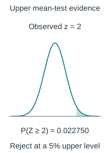
Worked upper mean test — For the fictional normal population with known σ=12, random independent sample n=36 and x̄=104, test H₀:μ=100 against μ>100. The upper-tail p-value P(Z≥2)≈0.02275013195 rejects at 5%. There is evidence of a higher population mean under those sampling and variance assumptions.The fictional known-variance mean example has null mean one hundred, population standard deviation twelve and sample size thirty-six. An observed average 104 is two standard errors above the null, giving upper-tail probability approximately 0.02275013195. The horizontal axis uses standardised z at 35 pixels per unit, with density scaled vertically by 600. The tail extends beyond the finite plotting window.
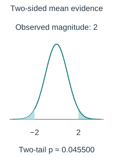
Worked two-sided mean test — For the same data but alternative μ≠100, the symmetric two-tail p-value is approximately 0.04550026390. This still rejects at 5% but not at 1%. The alternative controls the tail calculation even though the observed mean and standardised score have not changed.For the same observed magnitude two but a two-sided normal mean alternative, both extreme tails beyond plus and minus two are counted. Each has area approximately 0.02275013195, giving total p approximately 0.04550026390. These are observed-evidence tails; the 5% critical-score boundaries are approximately plus/minus 1.959963985 instead.
Upper critical mean — At a 5% upper-tail level, the standard normal critical score is approximately 1.644853627. For null mean 100 and standard error 2, the critical sample mean is 100+2×1.644853627≈103.2897073. Compare the observed mean to that boundary; do not use the population standard deviation twelve in its place.
Two-sided critical means — For a two-sided 5% normal mean test, reject when |Z|≥1.959963985 approximately. In the same null model this is X̄≤96.08007203 or X̄≥103.9199280. Each null tail has area 0.025; the region outside those boundaries has total area 0.05 before rounding effects.
Effect of sample size — Under the fixed known-σ model, increasing n reduces standard error as 1/√n. Quadrupling n halves it. This makes a given mean difference correspond to a larger |z|, but cannot repair selection bias, dependence or a wrong population variance assumption. Statistical detectability and practical importance remain separate.
Units and checking — The observed mean, null mean and σ must use compatible units, while Z is dimensionless. If variance is supplied, take its square root before dividing by √n. Draw the relevant tail, retain guard digits and compare the resulting probability or critical value with the originally specified level.
Evaluating and communicating test conclusions
Not proof of the null — An observation outside the critical region does not prove an exact population claim. The sample may simply lack enough evidence for the specified alternative at the chosen level. Use insufficient evidence wording and avoid asserting a probability that the null is true without an appropriate separate framework.
Not practical importance — A statistically significant difference can be small in its subject context, while a practically important difference may not cross a statistical threshold in a noisy or limited sample. Report the estimated direction and scale alongside the test and assess why it matters in the stated setting.
Error interpretation — A model-true null can still produce an unusual observation and be rejected. The nominal or actual significance level describes that long-run chance for the procedure under H₀; it is not a statement that this particular completed decision is known to be wrong with that probability. Formal additional error classifications are not required here.
Repeated testing choices — Testing many outcomes or repeatedly looking until a threshold is crossed can produce more false alarms than a single prespecified test. The elementary level refers to the defined procedure, so document the original question, sample and decision rule. Do not claim a single-test error guarantee for an altered exploratory process.
Complete test argument — Define the population parameter, state hypotheses and assumptions, identify the null distribution and statistic, show the correct evidence calculation, compare at the chosen level and give a contextual conclusion. Check model suitability and whether a reported probability is exact within a model, an approximation or a supplied result.
Test yourself
50 questions · Random sets of 10. These quick checks support revision; practise longer explanations and justified judgements too.
 Mr Kidman's Classroom