Charge and carriers — Electric charge Q is measured in coulombs. Electrons have charge −e, with e approximately 1.60 × 10⁻¹⁹ C; ions or other particles can also carry charge. A current requires net transport of charge, not necessarily electrons moving through every type of conductor.
Current as a rate — Current I = ΔQ/Δt is the average rate of charge flow through a cross-section, in A or C s⁻¹. A steady 0.20 A transfers 0.20 × 30 = 6.0 C in 30 s. For varying current the transferred charge is the signed area under an I-time graph; use a consistent direction convention.
Conventional direction — Conventional current is the direction positive charge would move. In a metallic wire, electron drift is opposite that direction. Drift means the slow average motion of charge carriers, superimposed on their random motion. The field is established around a circuit far more rapidly than individual carriers drift along it; electrons do not have to travel from the cell to the bulb before the bulb begins responding.
Potential difference — Potential difference V between two points is energy transferred per unit charge, V = W/Q, measured in volts or J C⁻¹. A 6.0 V component transfers 18 J when 3.0 C passes. Voltage is between points rather than a substance used up in the wire.
Junction conservation — Charge conservation implies that total current entering a junction equals total current leaving it when charge is not accumulating. A 0.80 A input splitting into 0.30 A and a second branch gives 0.50 A in that branch. Charges are not consumed by a resistor; electrical energy is transferred while charge continues to flow.
Loop energy balance — Around a complete circuit loop the energy gained per unit charge from sources equals energy transferred per unit charge elsewhere. Include source polarities and use a consistent traversal direction. In a simple series network the potential differences across resistive components add to the supply's terminal potential difference.
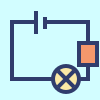
Circuit measurement — An ammeter is placed in series with the branch whose current is measured and ideally has negligible resistance. A voltmeter connects across two points and ideally has very large resistance. Real instruments can alter circuit current because they draw current or add resistance; this effect is called loading; never connect a low-resistance ammeter directly across a cell as a voltage measurement.
Resistance networks and power
Resistance definition — Resistance R = V/I relates the potential difference across a component to its current at a particular operating point, in ohms Ω. The definition does not require R to be constant. On a nonlinear I-V graph, V/I at a point is not generally equal to the tangent slope or its reciprocal.
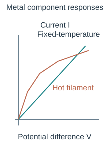
Ohmic condition — An ohmic conductor has I proportional to V while relevant physical conditions, particularly temperature, remain constant. Its I-against-V graph is straight through the origin with gradient 1/R. Heating a metal changes resistance, so a component can be ohmic under controlled conditions but show a curved measured graph when heating is significant.
Series derivation — Resistors in series carry the same current by charge conservation. Energy conservation gives Vtotal = IR₁ + IR₂ + …, so Rtotal = R₁ + R₂ + …. Adding a series resistor increases total resistance and reduces current for a fixed ideal supply. The current does not decrease successively through the series resistors.
Parallel derivation — Parallel branches share a potential difference V. Their currents add, so Itotal = V/R₁ + V/R₂ + … and 1/Rtotal = 1/R₁ + 1/R₂ + …. Equivalent resistance is smaller than the smallest branch resistance because a parallel branch supplies an extra conducting path.
Mixed network example — A 6 Ω resistor in parallel with 3 Ω gives Rp = (1/6 + 1/3)⁻¹ = 2 Ω. If this pair is in series with 4 Ω, total resistance is 6 Ω. Across an ideal 12 V supply total current is 2 A, the pair has 4 V across it, and branch currents are 2/3 A and 4/3 A.
Power derivation — Energy per charge is V and charge per time is I, so electrical power P = VI. For steady conditions W = VIt. Substituting V = IR gives P = I²R or P = V²/R, using the appropriate operating resistance. These alternatives predict different effects if the controlled quantity is current rather than voltage.
Power and supply comparison — At fixed voltage, doubling an ohmic resistance halves power V²/R; at fixed current it doubles power I²R. A 6.0 Ω resistor carrying 0.50 A dissipates 0.50² × 6.0 = 1.5 W and transfers 90 J in 60 s. Check the component's safe power rating rather than treating any mathematical current as experimentally acceptable.
Components resistivity and microscopic transport
Metal I-V response — A metal resistor held at constant temperature has a straight I-V graph. A filament lamp heats as current increases; more lattice vibration increases scattering, so resistance rises and the I-V curve becomes shallower at larger magnitude of V. A reverse voltage reverses current in a symmetric filament under corresponding steady conditions.Positive-quadrant schematic I-V responses contrast a temperature-controlled ohmic conductor with a filament that heats as voltage rises. The nonlinear filament curve becomes shallower. No universal numerical characteristic or negative-bias diode behaviour is asserted.
Diode response — A diode conducts strongly for one polarity once forward potential is sufficient for appreciable conduction, and normally carries very little reverse current within its safe range. Its forward I-V curve is strongly nonlinear. The apparent turn-on value depends on device and current; do not claim every diode has one universal exact threshold.
Thermistor response — For a negative-temperature-coefficient thermistor, heating greatly increases the number of available charge carriers, reducing resistance over the operating range. A fixed-temperature resistance measurement differs from a large-current I-V sweep that self-heats it. Explain which conditions change instead of describing every thermistor as a metal resistor with the same temperature trend.
LDR response — A light-dependent resistor has lower resistance when more suitable illumination generates additional mobile carriers. At fixed supply voltage its current therefore rises as it becomes brighter within its operating range. Light intensity, spectrum and temperature can affect calibration, so a particular sensor output needs measurement rather than an invented universal scale.
Resistivity definition — For a uniform specimen, R = ρl/A, where resistivity ρ has unit Ω m and depends on material and conditions. A longer wire has more resistance; a wider wire provides more conducting cross-section. Resistance is a property of the specimen; resistivity separates material behaviour from geometry.
Resistivity calculation — A 1.00 m wire of diameter 0.50 mm has area A = πd²/4 = 1.9635 × 10⁻⁷ m². If R = 2.0 Ω, ρ = RA/l = 3.93 × 10⁻⁷ Ω m. Squaring the diameter in millimetres without converting the area to m² would give a large error.
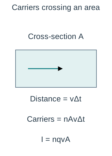
Drift-current derivation — In time Δt, carriers with drift speed v move through a cylinder of volume AvΔt at a cross-section. With number density n, the number of carriers per unit volume, and charge magnitude q, the transported charge magnitude is nAvΔt q, giving I = nqvA for a single carrier type. Here n is per m³ and v is drift speed, not random thermal speed.The schematic swept volume has length v times delta t and conducting cross-section A. Multiplying its volume by carrier number density counts carriers, then multiplying by charge and dividing by time gives I = nqvA. The arrow is net drift, not random thermal motion.
Microscopic interpretation — For fixed current and area, a lower carrier density needs a larger drift speed. Metals have many mobile conduction electrons; increasing temperature usually increases lattice scattering and resistance. In a semiconductor sensor, the large change in carrier number can dominate the temperature or illumination response. Carrier density alone is not the only determinant of resistivity.
CP2 apparatus and controls — Measure the potential difference across a known length of wire and the current through it, then R = V/I. Measure diameter at several positions and orientations with a zero-checked micrometer, and measure length between the actual electrical contact points. Keep current low or switch off between readings to limit temperature rise.
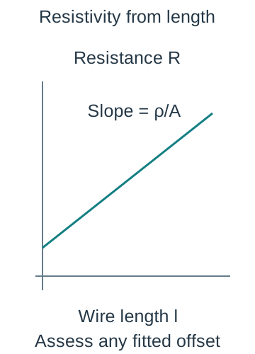
CP2 graphical processing — Vary wire length while material, diameter and temperature remain approximately constant; plot resistance against length. The ideal gradient is ρ/A, so ρ = gradient × A. A nonzero intercept may reveal contact or lead resistance, but distinguish whether the voltage contacts actually include those resistances before claiming the intercept's cause.Resistance plotted against actual measured specimen length gives gradient resistivity divided by area in the uniform fixed-temperature model. An offset is shown to emphasise that it needs measurement-specific interpretation rather than automatic forced-zero fitting.
CP2 uncertainty and safety — Since ρ = Rπd²/(4l), diameter percentage uncertainty contributes twice under a conservative rule; include resistance or gradient and length contributions without double counting. Longer lengths can improve the fractional length resolution but also raise resistance. Avoid touching hot wire, limit power and keep connections secure under the school method.
Potential dividers and sensors
Uniform wire potential — For a uniform wire at steady current and constant temperature, resistance is proportional to length, so potential difference along it is proportional to distance. The potential gradient V/l is constant under these assumptions. Poor contacts, nonuniform cross-section or heating can make a real wire depart from this model.
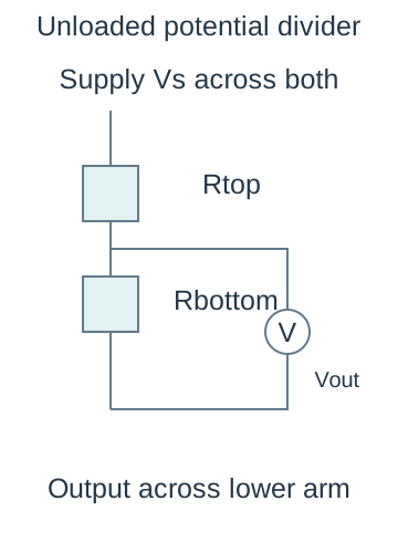
Divider derivation — Two series resistors Rtop and Rbottom across a supply Vs carry I = Vs/(Rtop + Rbottom). Output across the lower resistor is Vout = IRbottom = VsRbottom/(Rtop + Rbottom). Specify which component is the output: exchanging them changes the response even though total current is unchanged.The two resistor arms are in series between supply terminals. Output is measured across the lower arm by a negligibly loading voltage input; the branch outline marks the measured nodes, not a conducting short. A finite load would need a parallel equivalent.
Divider example — A 2.0 kΩ top resistor and 3.0 kΩ lower resistor across 10 V give I = 10/5000 = 2.0 mA and output 6.0 V across the lower resistor. The formula assumes that the output device draws negligible current and that the source maintains its voltage.
Loading a divider — Connecting a load RL across Rbottom replaces that arm with Rbottom in parallel with RL. Its effective resistance decreases, so output falls for a fixed upper resistor and supply. Use the effective parallel value in the divider calculation rather than applying the unloaded formula after attaching a low-resistance load.
NTC placement and response — NTC means negative temperature coefficient: resistance falls as temperature rises over the working range. With an NTC thermistor in the lower arm, warming reduces its resistance and lowers Vout. With the thermistor in the upper arm and a fixed lower resistor, warming reduces the denominator while the numerator stays fixed, so Vout rises. State the placement and the measured output before describing a thermostat's signal.
Light-sensor divider — For an LDR in the lower arm, brighter illumination reduces its resistance and output; for an upper-arm LDR, brighter illumination raises output across a fixed lower resistor. A switching circuit may respond when the calibrated output crosses a chosen threshold, but no universal light level follows from the divider equation alone.
Sources emf and internal resistance
Emf and terminal voltage — Electromotive force ε is the energy supplied by a source per unit charge, measured in volts despite the word force. Terminal potential difference is energy transferred per charge to the external circuit. In a discharging cell with internal resistance r, ε = V + Ir, so V = ε − Ir.
Internal energy transfer — With current I, internal power dissipation is I²r. The cell's total supplied power εI splits into external VI plus internal I²r. Open circuit ideally gives I ≈ 0 and V ≈ ε; real voltmeters draw a small current. An open-circuit reading does not determine internal resistance by itself.
Loaded-cell example — A cell of ε = 1.50 V and r = 0.50 Ω supplies an external 2.50 Ω resistor. Current is 1.50/(2.50 + 0.50) = 0.50 A and terminal voltage is 0.50 × 2.50 = 1.25 V. The lost volts are 0.25 V, meaning internal energy transfer per charge, not disappearance of charge.
Changing external load — Reducing external resistance increases current and the internal voltage drop, lowering terminal voltage for a fixed ε and r model. The ideal short-circuit expression I = ε/r is a limiting calculation, not an experimental instruction: excessive current can heat and damage a source. Real ε and r can also vary with temperature, state and time.
CP3 measurement — Connect an ammeter in series with a variable load and a voltmeter across the cell terminals. Take simultaneous V and I readings over a safe range, limiting discharge time and heating. Include an open-circuit point where feasible, but obtain multiple loaded points to determine both model parameters.
CP3 graph and interpretation — Plot terminal V vertically against I horizontally. A straight fit gives intercept ε and negative gradient −r. Two illustrative points (0.10 A, 1.45 V) and (0.50 A, 1.25 V) imply gradient −0.50 Ω and intercept 1.50 V. Use a fit across the data and assess uncertainty rather than relying on one pair alone.The constant-emf, constant-internal-resistance cell model gives a terminal-voltage line with intercept emf and negative slope internal resistance. This is a schematic model to test with actual simultaneous readings and uncertainty.
CP3 evaluation — A cell that warms or discharges substantially can drift during the sequence. Switch off between readings, repeat a reference load or vary order to detect drift, and avoid unstable contacts. A curve in V against I may challenge the constant-parameter model. Quote justified gradient/intercept uncertainty and do not force a preferred textbook emf.
Test yourself
50 questions · Random sets of 10. These quick checks support revision; practise longer explanations and justified judgements too.
 Mr Kidman's Classroom