Density and scale — Density ρ = m/V is mass per unit volume, measured in kg m⁻³. It is a property of the material under specified conditions, not a measure of the mass of an object alone. A large low-density block can have more mass than a small high-density bead. State temperature where expansion could change the volume appreciably.
Volume conversions — Convert a volume by cubing the length conversion: 1 cm³ = 10⁻⁶ m³, so 1 g cm⁻³ = 1000 kg m⁻³. Treating cm³ as 10⁻² m³ introduces a factor of ten thousand error. For a cylinder use V = πd²l/4 with all lengths in metres before calculating its density.
Density worked method — An illustrative solid of mass 0.156 kg displaces 20.0 cm³ of water. Its volume is 20.0 × 10⁻⁶ m³, so ρ = 0.156/(20.0 × 10⁻⁶) = 7800 kg m⁻³. Record the initial and final cylinder readings and ensure full immersion; trapped bubbles would overestimate solid volume and underestimate density.
Density measurement choices — Use a balance and geometric dimensions for a regular solid, or displacement for an insoluble irregular solid. A liquid's mass is the difference between filled and empty container readings at the chosen volume. Choose apparatus that resolves the actual change well; a coarse measuring cylinder is unsuitable for a very small bead's individual volume.
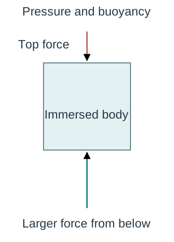
Origin of upthrust — Fluid pressure increases with depth, so the upward pressure force on the lower surface of an immersed object exceeds the downward force on its upper surface. The resultant is upthrust. For a wholly or partly submerged object it equals the weight of displaced fluid, not automatically the object's own weight.A schematic immersed body experiences a larger upward pressure force at its deeper lower face than the downward force at its top. Horizontal fluid forces cancel in this symmetric drawing. Weight is not included in this pressure-only explanation; it must be added in the complete body force diagram.
Archimedes calculation — For displaced volume V in fluid of density ρf, U = ρfVg. An immersed 2.0 × 10⁻⁵ m³ object in water of density 1000 kg m⁻³ experiences U = 1000 × 2.0 × 10⁻⁵ × 9.81 = 0.1962 N. This buoyancy acts upward even if the object sinks; sinking means its weight exceeds the other upward forces.
Floating equilibrium — For a floating object at rest, upthrust equals weight, giving ρfVsubg = mg. If the object has uniform average density ρo and total volume Vo, Vsub/Vo = ρo/ρf. A 600 kg m⁻³ block floats with 60% of its volume under water of density 1000 kg m⁻³, ignoring surface tension.
Apparent weight — A force meter supporting a fully immersed stationary object reads T = mg − U when no other vertical forces act. Its mass has not changed: the reading is a support force. Weighing in air and liquid can determine displaced volume, but contact with the container or a surface-tension force at a narrow suspension needs consideration.
Viscosity drag and falling spheres
Viscous resistance — Viscosity describes resistance to relative motion between neighbouring fluid layers. In a simple shear model, dynamic viscosity η links shear stress (sideways force per unit area between layers) to velocity gradient (how rapidly flow speed changes across the layers); its SI unit is Pa s, equivalent to kg m⁻¹ s⁻¹. It differs from density and from the drag force on a particular moving object.
Laminar and turbulent flow — In laminar flow fluid layers move smoothly without irregular mixing. Turbulence involves fluctuating eddies, irregular swirling regions of fluid, and changes the drag relationship. Slow motion alone is not a universal guarantee of laminar flow: object size, density and viscosity matter too. The stated Stokes model assumes a small sphere moving slowly through a continuous fluid.
Stokes law and conditions — The magnitude of viscous drag on a sphere in the Stokes regime is D = 6πηrv, opposite its velocity relative to the fluid. Here r is radius rather than diameter and v is relative speed. Use a sphere small compared with its container, slow enough to avoid turbulence and far enough from walls for boundary effects to be small.
Drag calculation — For η = 0.80 Pa s, r = 1.0 × 10⁻³ m and v = 0.020 m s⁻¹, D = 6π × 0.80 × 1.0 × 10⁻³ × 0.020 = 3.02 × 10⁻⁴ N. The force is not a material constant: it changes with radius and speed as well as viscosity. Convert millimetres to metres before substitution.
Three-force model — A sphere falling through a liquid has weight mg downward, buoyancy U upward and viscous drag D upward. Initially its small speed gives small drag, so if mg > U it accelerates downwards. As speed rises drag rises, reducing the downward resultant and acceleration. Draw these forces on the sphere, not a fictitious downward force called motion.
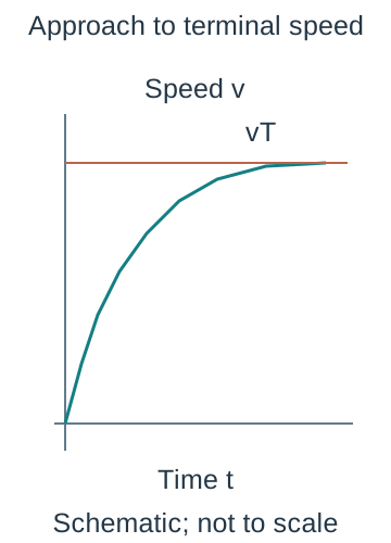
Terminal motion — At terminal speed vT, mg = U + D and acceleration is zero while velocity remains nonzero. The force balance does not mean that weight or drag vanishes. A denser sphere released in a viscous liquid approaches this state after an initial transient; measure between markers only after its speed is steady.At steady downward motion, sphere weight is balanced by upward drag plus upthrust. The three arrows identify the separate forces; their lengths are schematic rather than a calibrated force scale. Nonzero terminal velocity is compatible with zero acceleration.
Deriving terminal speed — Use m = ρs(4πr³/3), U = ρf(4πr³/3)g and D = 6πηrvT in the terminal force balance. Cancelling πr gives vT = 2r²g(ρs − ρf)/(9η). This equation includes buoyancy. Omitting ρf is justified only if the fluid density is negligible compared with the sphere's density.
Finding viscosity — Rearrange to η = 2r²g(ρs − ρf)/(9vT). For r = 0.50 mm, ρs = 7800 kg m⁻³, ρf = 1200 kg m⁻³ and vT = 0.0040 m s⁻¹, η = 0.899 Pa s to three significant figures. The calculation assumes steady Stokes flow and an effectively unbounded liquid, so it is a model-based determination.
Radius dependence — For spheres of the same material in the same liquid at fixed temperature, vT ∝ r² within the Stokes regime. Plot vT against r² to test the relationship; a straight line through the origin supports the model. Doubling radius predicts four times the terminal speed only while the larger sphere still satisfies the model conditions.
Temperature dependence — For a typical liquid, dynamic viscosity decreases as temperature rises. Keep the bath temperature steady and report it, since warming by handling or room changes can alter terminal speeds. Gas viscosity can behave differently; avoid claiming that all fluids have the same temperature trend.
CP4 apparatus and measurement — Measure the sphere diameter in several orientations with a micrometer, halve the mean to obtain r, and measure a clearly marked vertical separation s below the initial acceleration region. Release into a deep transparent liquid column without imparting a sideways push. Time its motion through s, using video or suitable sensors where manual timing is too coarse.
CP4 verifying terminal speed — Use several equal marker intervals down the column. Equal traversal times within measurement uncertainty support constant speed, so vT = s/t is appropriate. Move the timed region lower if successive intervals become faster. A long single interval alone cannot show that the sphere was terminal throughout it.The schematic speed-time curve approaches a horizontal terminal-speed reference from below. Its initially positive gradient decreases towards zero. Equal timings over equal successive distances are an experimental check of steady motion, not a consequence of merely choosing a long interval.
CP4 control and safety — Use a wide column, keep the sphere near the centre, avoid bubbles and maintain temperature. Secure the vessel and contain spills because a viscous liquid on the floor is a slip hazard. Retrieve spheres without reaching into unsafe apparatus or cracking glass. School-approved handling of the chosen liquid is required; revision does not replace its risk assessment.
CP4 uncertainty and bias — Because η ∝ r²/vT and vT = s/t, a worst-case percentage estimate adds twice the radius percentage uncertainty to those for distance and time, with density uncertainties included if significant. Repeats reduce random timing scatter but do not remove wall drag, a zero error or a wrong density. Wall-enhanced drag lowers vT and can make the inferred η too high.
Deformation and material behaviour
Extension and compression — Extension x is loaded length minus original length; it is not the total length. A tensile force stretches a specimen and a compressive force shortens it. For a small compression one may use positive magnitudes, but any signed force-displacement equation must state its axis and distinguish applied force from the restoring force.
Stiffness and Hooke — In the proportional region ΔF = kΔx, where stiffness k has units N m⁻¹. With the reference chosen at zero force and zero extension this becomes F = kx. A 15 N load giving 3.0 mm extension has k = 15/0.0030 = 5000 N m⁻¹. Hooke's law is a restricted material response, not a universal law for every deformation.
Force-extension gradient — On a graph with force vertically and extension horizontally, the proportional straight-line gradient is k. If the axes are exchanged the gradient is 1/k. Include units and use a large gradient triangle on the best-fit line, rather than a single noisy point whose ratio can be distorted by an offset.
Proportionality versus elasticity — The limit of proportionality is where force ceases to be proportional to extension. The elastic limit is the greatest loading from which the specimen fully recovers its original dimensions when unloaded. A material may have a nonlinear but reversible region between them, so the two limits need not coincide.A force-extension sketch marks the end of the initial proportional straight segment. The later curve can remain reversible, but that requires unloading evidence; the drawing alone does not locate the elastic limit or claim that every material has the same curve.
Elastic deformation — Elastic deformation is reversible after unloading. In the ideal linear region unloading retraces the loading line and all stored strain energy can be returned. Real reversible materials may show some energy dissipation; elastic does not by itself guarantee a perfectly straight graph or zero heating in a load-unload cycle.
Plastic deformation and yield — Plastic deformation leaves a permanent change after unloading. Around yield, large extra strain can occur for a small increase in stress for some materials; the detailed shape is material dependent. A specimen can remain intact after yielding. Do not identify the yield point with the breaking point or with the initial proportionality limit.
Ductile and brittle response — A ductile material can undergo substantial plastic extension before fracture; a brittle material breaks with little plastic strain. A strong material withstands high stress, while a stiff material has a large elastic stress/strain ratio. These properties are distinct: a material can be stiff yet brittle, and a compliant material, which deforms readily under load, may absorb substantial energy before breaking.
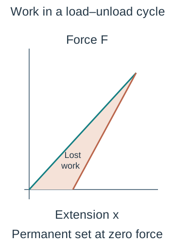
Loading and unloading evidence — An unloading line that reaches zero force at positive extension indicates a permanent set. The area between loading and unloading curves is energy dissipated during that cycle. It is not simply the maximum energy supplied. Identify the axes and compare curves over the same complete loading history before describing hysteresis.
Geometry changes stiffness — For a uniform wire of Young modulus E, original length L and area A, F/x = EA/L in the linear elastic region. Increasing length lowers stiffness; increasing cross-sectional area raises it. These changes do not change the intrinsic Young modulus of the same material at the same conditions.
Stress strain and Young modulus
Tensile stress — Engineering tensile stress σ = F/A uses the original cross-sectional area and has units Pa, or N m⁻². The same force produces greater stress in a thinner wire. Distinguish this average stress from local concentrations near defects, clamps or notches, where failure may begin.
Tensile strain — Engineering strain ε = x/L is change in length divided by original length and has no unit. A 2.0 m wire extended by 1.0 mm has strain 0.0010/2.0 = 5.0 × 10⁻⁴, or 0.050%. An extension in metres alone is not a strain, and using the final length changes the defined quantity.
Young modulus definition — Young modulus E = σ/ε = FL/(Ax) in the linear elastic region. Its unit is Pa, and it is the gradient of a stress-against-strain graph there. After the proportional region, the ratio or local slope need not equal the original Young modulus. Capital E here is a modulus, not the energy symbol used in other contexts.
Modulus worked method — A 2.00 m wire of diameter 0.50 mm extends 1.00 mm under 20.0 N. A = π(0.00050)²/4 = 1.9635 × 10⁻⁷ m², so stress = 1.0186 × 10⁸ Pa and strain = 5.00 × 10⁻⁴. Thus E = 2.037 × 10¹¹ Pa, about 2.0 × 10¹¹ Pa at the diameter's precision.
Stress-strain graphs — Plot engineering stress against strain to compare material behaviour independently of initial specimen dimensions. The initial gradient gives E, the extent of plastic strain indicates ductility, and the stress at fracture is breaking stress. A maximum stress before fracture can differ from the breaking stress as necking, a local narrowing of the specimen, changes its geometry.An illustrative engineering stress-strain curve shows a steep elastic region, a yield region, later rising stress and eventual fracture after substantial plastic strain. The stress uses original area. The detailed shape and the separation of maximum stress from fracture are material dependent; neither axis has a numerical scale.
Compression and comparison — Stress and strain can also describe compression using a stated sign convention or magnitudes. A compressive modulus determination still needs a suitable linear response and uniform loading; a long thin specimen can buckle rather than undergo uniform compression. Do not apply a tensile curve to an unrelated geometry without checking the deformation model.
CP5 loading arrangement — Clamp a long fine wire securely and add measured loads in small increments. Measure the original gauge length L, the length of the wire section whose extension is measured, and the corresponding extension with a pointer, travelling microscope or suitable displacement sensor. A small initial tension removes slack; define how the baseline load and extension are accounted for rather than treating slack straightening as elastic extension.
CP5 diameter and reference — Measure diameter with a micrometer in several positions and orientations, checking its zero and using its ratchet to avoid excessive force. A = πd²/4 makes diameter precision especially important. A reference wire or stable reference marker can help separate support motion and thermal changes from the test wire's extension.
CP5 processing — Plot F against x and determine its linear gradient k, then E = kL/A. Alternatively plot stress against strain and use the linear gradient directly. Take sufficient loading points, repeat where safe, and unload to check reversibility. Do not fit the plastic region with the elastic line simply to increase the number of points.
CP5 uncertainty — For E = 4FL/(πd²x), a worst-case fractional estimate is ΔE/E ≈ ΔF/F + ΔL/L + 2Δd/d + Δx/x. If the measured gradient replaces F/x, use its assessed uncertainty instead of counting F and x again. Longer gauge length increases extension for the same stress and reduces the relative effect of a fixed extension resolution.
CP5 safety and evaluation — Wear eye protection where a loaded wire could snap, shield the wire as appropriate, secure clamps and keep feet and the bench clear of falling masses. Do not exceed the safe working range to locate fracture during a modulus determination. Explain a specific limitation such as clamp slip and its direction of effect, rather than writing human error as an evaluation.
Strain energy and model evaluation
Work during stretching — For a small extra extension dx, work transferred by a slowly applied tensile force is approximately F dx. Adding the contributions gives the area under the force-extension curve. This method remains useful for a nonlinear loading curve; only a straight line through the chosen zero produces the simple triangular expression.
Linear elastic energy — When F increases linearly from zero to its final value, stored elastic energy U = ½Fx = ½kx². The factor ½ arises because the average loading force is half its final value. A spring of k = 250 N m⁻¹ extended 0.080 m stores ½ × 250 × 0.080² = 0.80 J, while its final force is 20 N.The shaded triangular area under a straight force-extension loading line is one half of final force times extension. This equals stored energy for ideal reversible linear loading from the stated zero. The diagram does not apply that triangle rule to a nonlinear curve.
Nonlinear area estimate — For illustrative extension values 0, 0.010 and 0.020 m with forces 0, 2 and 6 N, two trapezia give work ≈ ½(0 + 2)0.010 + ½(2 + 6)0.010 = 0.050 J. Using ½Ffinalxfinal gives 0.060 J and incorrectly assumes a straight line. Smaller intervals improve the graphical approximation for smooth curves.
Energy returned and dissipated — For a load-unload cycle, area under the unloading curve is work returned to the surroundings. The difference from the loading area is dissipated, commonly as internal energy and sound or in permanent structural change. A large area under a fracture curve means large work per specimen before failure, not automatically a large Young modulus.The green loading and brown straight unloading paths enclose the work dissipated in this illustrative plastic load-unload cycle. The positive zero-force extension indicates a permanent set. The area beneath the unloading line is returned work, while the full loading area is supplied work. Axes and paths are schematic.
Stress-strain energy density — Because F = σA and dx = L dε, dividing work by original volume AL gives energy density equal to the area under the stress-strain curve. In a linear elastic model this is ½σε = σ²/(2E). Its units Pa are equivalent to J m⁻³. Compare total energy only after considering specimen volume.
Model-based selection — Choose a material using the relevant combination of stiffness, strength, ductility, density and energy absorption, together with service conditions and evidence. A bridge cable may need high tensile strength and controlled extension, whereas an impact absorber benefits from dissipating energy without dangerous brittle fracture. A single label such as strongest cannot resolve every engineering decision.
Linking uncertainty to conclusions — When two modulus estimates overlap within their justified uncertainties, the data may not resolve a difference. This does not prove that the materials are identical. Report the assumptions behind the uncertainty estimate, identify systematic effects separately, and say what additional measurement would distinguish the proposed explanations.
Test yourself
50 questions · Random sets of 10. These quick checks support revision; practise longer explanations and justified judgements too.
 Mr Kidman's Classroom