Nuclear binding — Binding energy is the energy needed to separate a nucleus fully into its free nucleons. A bound nucleus has less rest mass than the same free nucleons; the difference Δm is the mass deficit, with binding energy ΔE = c²Δm. Binding does not mean nucleons vanish or that a nucleus contains no internal motion.
Mass accounting — For nuclear masses use Z proton masses plus (A − Z) neutron masses minus nuclear mass. If using neutral atomic masses, account consistently for electrons, often using hydrogen-atom masses with atomic nuclear-species masses. Do not subtract a neutral atom's mass from bare proton and neutron totals without addressing the extra electron masses.
Atomic mass unit — The unified atomic mass unit u is one twelfth of a carbon-12 atom's mass, approximately 1.66 × 10⁻²⁷ kg. Its energy equivalent is approximately 931.5 MeV per u. Use the supplied data precision and keep mass units distinct from energy units; a deficit in u must be converted before multiplying by c² in SI.
Binding worked example — An illustrative mass deficit 0.020 u corresponds to 0.020 × 1.66 × 10⁻²⁷ = 3.32 × 10⁻²⁹ kg. With c = 3.00 × 10⁸ m s⁻¹, binding energy is 2.99 × 10⁻¹² J, about 18.6 MeV. For A = 4 the binding energy per nucleon is about 4.66 MeV, not the total 18.6 MeV.
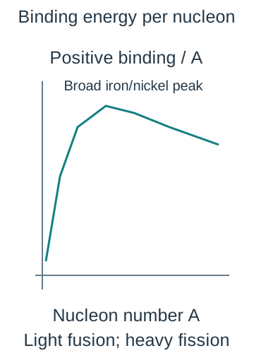
Binding curve — Plot positive binding energy per nucleon against nucleon number. It rises steeply among light nuclei, reaches a broad maximum around the iron/nickel region and decreases slowly for very heavy nuclei. Greater binding per nucleon generally means a more tightly bound nucleus; compare total before-and-after binding for an actual reaction rather than only one plotted point.The qualitative positive binding-energy-per-nucleon curve rises among light nuclei to a broad iron/nickel maximum then falls slowly for heavy nuclei. Actual reaction release requires comparing complete reactant and product totals, not simply reading one point.
Fission energy — Splitting a suitable heavy nucleus into medium-mass fragments can increase total binding energy and lower total rest mass, releasing the difference as fragment kinetic energy, neutron energy and radiation. Neutron-induced fission can also release further neutrons. Balance proton and nucleon numbers for a specified channel; there is no single universal fragment pair.
Chain reaction — If sufficient released neutrons cause subsequent fissions, the reaction can sustain a chain. Absorption, escape, geometry and material conditions determine whether it dies away, is steady or grows. A moderator can reduce neutron energies in suitable reactor designs and control absorbers reduce the population; these are distinct roles and not required in identical form for every reactor type.
Fusion and conditions — Combining sufficiently light nuclei into more tightly bound products can release energy. Positive nuclei repel electrically, so high temperatures give energetic collisions and high density increases collision opportunity. Confinement must keep suitable conditions long enough; temperature alone is not a complete practical reactor criterion, and not every possible nuclear combination releases energy.
Energy and risks — Nuclear energy calculations compare full reactant and product masses, including emitted particles. Decisions about fission and fusion also involve containment, radiation, materials, waste, fuel supply and evidence about the actual technology. A small mass change can release large energy through c², but that does not make the engineering or environmental comparison reducible to one number.
Radiation properties and nuclear equations
Background sources — Detectors register environmental radiation from cosmic sources, rocks and buildings, radon and other natural or human-made sources. Measure the background under comparable conditions without the experimental source. Subtract its count rate, not a raw count measured over a different time, from the source-plus-background rate.
Alpha beta gamma — Alpha particles are helium nuclei, beta-minus particles are electrons and gamma radiation is electromagnetic photons. Beta-plus particles are positrons. They differ in charge, rest mass, ionisation and penetration; radiation names identify what leaves the nucleus, not a claim that all charged products have identical ranges.
Ionisation and range — Alpha radiation strongly ionises over a short path and is stopped by paper or the outer skin layer, while beta has intermediate penetration and gamma is generally more penetrating and weakly ionising per path length. Actual range or attenuation depends on energy and material. A highly penetrating radiation can still interact and deposit energy in tissue.
Exposure and containment — An external alpha source may be stopped before reaching sensitive tissue, yet inhaled or ingested alpha emitters can be hazardous because energy is deposited internally. Risk depends on activity, radiation, exposure route, duration and shielding. Use the school's authorised procedures, minimise exposure time, maximise appropriate distance and use suitable shielding; never handle sources casually from a revision description.
Nuclear equation balances — In a nuclear transformation, sum nucleon numbers and charges consistently across all products. Alpha emission lowers parent A by 4 and Z by 2. Gamma emission changes neither A nor Z but reduces nuclear excitation energy. Include a neutron's A = 1 and Z = 0 rather than treating all uncharged particles as having zero nucleon count.
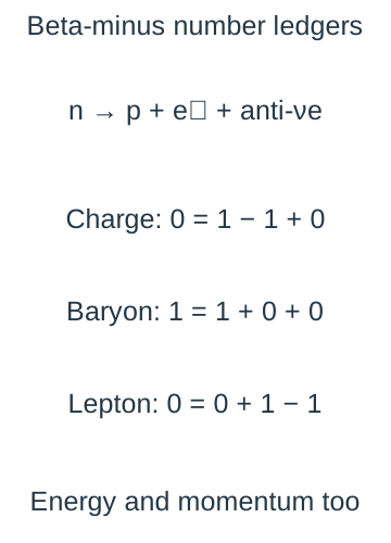
Beta transformations — In beta-minus decay a neutron becomes a proton with electron and antineutrino emission, so A stays fixed and Z rises by one. In beta-plus, a suitable proton-to-neutron transformation emits a positron and neutrino, lowering Z by one with unchanged A. The beta electron is created in the interaction, not pulled from the atomic electron shell.Independent charge, baryon and lepton ledgers explain the antineutrino partner in beta-minus transformation. The schematic uses relative electric charges and family counts, while full events must also conserve energy and vector momentum.
Random decay activity and half-life
Random and spontaneous — Spontaneous means decay occurs without needing an external trigger; random means the exact nucleus and time cannot be predicted. For a fixed isotope the probability per unit time is approximately constant under the course's ordinary conditions. Large populations show a predictable statistical trend even though individual events remain unpredictable.
Decay constant and activity — Decay constant λ is probability rate per undecayed nucleus in s⁻¹. Activity A = λN is the expected number of decays per second in Bq, while dN/dt = −λN expresses the decreasing population. The activity is positive; the negative sign belongs to the rate of change of N. Not every emitted quantum is detected.
Exponential law — For constant λ, N = N₀exp(−λt) and A = A₀exp(−λt) for a single isotope without a complicating daughter contribution. Count rate can follow the same form if detector efficiency and geometry stay fixed and background is corrected. A mixed source or evolving daughter can give a different observed curve.
Half-life derivation — At t½, N/N₀ = ½ = exp(−λt½), giving λ = ln2/t½. Each half-life halves the expected remaining population, not a fixed absolute number. After three half-lives the expected remaining fraction is 1/8 and decayed fraction is 7/8. A sample does not become exactly empty at a finite multiple in this continuous mean model.The schematic mean activity decreases exponentially for a single fixed decay constant after background correction. Individual counts still fluctuate and the curve is not a schedule for any particular nucleus.
Decay calculation — For half-life 120 s, λ = ln2/120 = 5.78 × 10⁻³ s⁻¹. An initial activity 800 Bq becomes 100 Bq after 360 s, while after 60 s it is 800exp(−ln2/2) = 566 Bq. The square-root-of-two factor at half a half-life differs from simply subtracting a quarter of the initial activity.
Graphical half-life — Subtract background, then determine repeated time intervals over which the fitted mean count rate halves. On a linear count-rate graph these intervals should agree within uncertainty for a single decay constant. A plot of ln corrected count rate against t has gradient −λ; use only positive corrected values and justify the chosen fit range.
Detection statistics — Counts fluctuate randomly; for a simple Poisson model expected standard count uncertainty is approximately √n for a sufficiently large observed count n. Fractional counting uncertainty then falls as 1/√n. Longer counting improves relative counting precision but can smear rapid decay over the interval; the detector also has efficiency, dead time (a short interval after a detection when the detector cannot register another event) and geometry limitations.
Background uncertainty — Subtracting a separately measured background rate does not remove its uncertainty. Include uncertainty from both source-plus-background and background measurements using the stated method. At weak source signals, a small difference between noisy counts can have large fractional uncertainty or even be negative; do not take its logarithm as if it were reliable positive activity.
Gamma absorption practical
CP15 geometry and controls — Use the approved source, detector and lead-absorber arrangement, keeping source-detector separation and alignment fixed. Record counts for a known time at each absorber thickness and take comparable background measurements. Handle lead with the school's hygiene controls and use authorised source tools and storage; minimise unnecessary exposure.
Attenuation model — For a narrow gamma beam of fixed energy, a simple model is I = I₀exp(−μx), where x is absorber thickness and μ is the linear attenuation coefficient in m⁻¹. It describes how strongly the beam is reduced per unit absorber thickness under the stated conditions; a larger μ gives a faster decrease with thickness. Absorption and scattering remove photons from the detected beam. Gamma radiation does not have one sharp stopping thickness analogous to an ideal fixed charged-particle range.
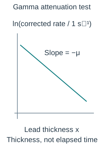
CP15 processing — Convert counts to rates, subtract background and plot ln corrected rate against measured lead thickness. A straight fit has gradient −μ and a half-value thickness ln2/μ. Keep source and detector geometry constant so inverse-square changes do not mimic attenuation. Half-value thickness is a length, not a radioactive half-life time.Logged positive corrected detector rate plotted against lead thickness gives slope minus attenuation coefficient in the simple fixed-energy narrow-beam model. This spatial law must not be confused with a radioactive half-life measured in time.
CP15 evaluation — Use repeated or longer counts where safe to reduce relative fluctuations, measure thickness accurately and avoid gaps or changed alignment. Scattered photons reaching the detector, mixed gamma energies, detector dead time and dominant background can bend the simple plot. More lead is not by itself a guarantee that a weak corrected point is statistically meaningful.
Evidence and model choice — Distinguish decay with elapsed time from attenuation with absorber thickness: both can be exponential but describe different processes and constants. Neither increasing shielding nor changing detector efficiency changes the source's intrinsic half-life in this course's model. Explain which quantity was measured and what assumptions connect it to activity or beam intensity.
Test yourself
50 questions · Random sets of 10. These quick checks support revision; practise longer explanations and justified judgements too.
 Mr Kidman's Classroom