Physical quantities — A physical quantity is expressed as a numerical value multiplied by a unit. Writing a speed as 12 is incomplete unless the context fixes its unit. Distinguish the quantity itself from a particular measurement and from its symbol: time t, for example, can be measured in seconds or converted from other time units.
SI base quantities — The seven SI base quantities and units are time second s, length metre m, mass kilogram kg, electric current ampere A, thermodynamic temperature kelvin K, amount of substance mole mol and luminous intensity candela cd. Do not replace kilogram with gram when constructing a base-unit expression.
Derived quantities — A derived quantity combines base quantities: velocity uses m s⁻¹, acceleration m s⁻² and force kg m s⁻². The newton N is a named derived unit, not an extra base unit. Deriving units from an equation provides a useful consistency check and clarifies whether a graph gradient has the expected physical meaning.
Dimensional checks — Since work is force times distance, a joule is kg m² s⁻²; power in watts is kg m² s⁻³. Dimensions describe which base quantities a quantity contains and to what powers; energy, for example, has mass × length² ÷ time². An equation cannot add quantities with different dimensions. Dimensional consistency is necessary but insufficient for correctness: it cannot determine a missing dimensionless factor such as ½ in kinetic energy.
Prefixes and powers — Prefixes multiply the whole unit: milli m means 10⁻³, micro μ means 10⁻⁶, nano n means 10⁻⁹, kilo k means 10³ and mega M means 10⁶. For area or volume, raise the conversion factor to the corresponding power. Thus 2.0 mm² = 2.0 × 10⁻⁶ m², not 2.0 × 10⁻³ m².
Standard form and orders — Write 0.000045 as 4.5 × 10⁻⁵. Dividing 6 × 10⁶ by 2 × 10⁻³ gives 3 × 10⁹ because the exponents subtract. An order-of-magnitude estimate focuses on scale, not spurious decimal precision. Make the convention clear if assigning a nearest power of ten.
Estimation as modelling — To estimate an unfamiliar quantity, identify a physical model and plausible inputs. A classroom of approximate dimensions 8 m by 6 m by 3 m has volume about 144 m³; taking air density as 1.2 kg m⁻³ gives air mass about 170 kg. This is a modelled estimate, not a measured property of the learner's actual room.
Sanity and significant figures — Check sign, scale, units and limiting behaviour before trusting a calculator. A runner's speed of 3000 m s⁻¹ suggests a conversion error. Keep extra unrounded digits, called guard digits, during calculations and round the final result to precision supported by data and uncertainties; trailing zeros or many displayed digits do not create accuracy.
Mathematical models and graphs
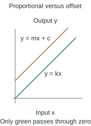
Proportionality and offsets — Direct proportionality y = kx produces a straight line through the origin. A straight line y = mx + c with nonzero c is linear but not directly proportional. For a spring experiment an offset can reflect the chosen preload reference or a systematic issue; it should be interpreted rather than automatically forced away.Two schematic straight lines distinguish direct proportionality through the origin from a linear response with a nonzero intercept. Neither graph claims experimental values; interpreting a fitted offset requires the actual measurement procedure.
Inverse and power models — An inverse relationship y ∝ 1/x is linearised, meaning represented as a straight-line graph, by plotting y against 1/x; y ∝ x² is tested by y against x². Transform the actual measured variable before plotting and identify the gradient's units. A graph's visual shape alone over a narrow range may not discriminate two competing models.
Best-fit practice — Put the independent variable horizontally and the dependent variable vertically unless a justified linearisation dictates otherwise. Label quantity and unit, choose scales using the available area and show suitable error bars. A best-fit line represents the trend; it need not pass through every measured point or the origin.
Gradient from data — For a straight-line gradient use two well-separated coordinates on the best-fit line, not necessarily raw observations. With force rising from 2.0 to 8.0 N as extension rises from 0.010 to 0.040 m, k = 6.0/0.030 = 200 N m⁻¹. Include units obtained from vertical units divided by horizontal units.
Curves and local rates — The gradient of a tangent gives an instantaneous rate, such as velocity from a displacement-time graph. A chord, the straight line joining two points on the curve, gives an average over an interval. Draw a suitably long tangent and large triangle to reduce reading uncertainty, while avoiding a triangle that no longer follows the tangent's actual slope.
Areas as accumulation — Graph area has units equal to vertical units multiplied by horizontal units. Area under velocity against time is signed displacement; the sum of absolute areas is distance travelled. For nonuniform data use appropriate interval widths in trapezia rather than assume equal spacing. An acceleration-time area gives velocity change.
Logarithmic power plots — For y = axⁿ with positive x and y, ln y = ln a + n ln x. Here ln means the natural logarithm, with base e; it reverses raising e to a power. For example, ln(e³) = 3. Strictly logarithms apply to numerical ratios to chosen reference units; keeping one unit convention throughout makes the slope n meaningful. The intercept determines a in that convention. A straight log-log line supports a power model over the tested range only.
Exponential linearisation — For y = y₀exp(−kt), ln y = ln y₀ − kt; a plot of ln y against t has gradient −k and intercept ln y₀. Subtract a known constant background before taking the logarithm if the physical model concerns the signal alone. Zero or negative corrected observations cannot be directly logged.The ideal logged discharge is a straight line of negative slope. The vertical axis explicitly logs the voltage ratio to one volt, and the physical fit requires positive background-corrected voltage. The schematic line is not a measured data set.
Interpolation and extrapolation — Interpolation estimates within the observed range; extrapolation extends beyond it and is more dependent on model validity. A component's near-constant resistance at small currents does not guarantee the same response after substantial heating. Give the physical reason for a restricted range instead of treating every straight fit as a universal law.
Measurement uncertainty and data treatment
Accuracy precision and resolution — Accuracy concerns closeness to a true or accepted value, precision concerns the spread of repeated values, and resolution is the smallest change the instrument distinguishes. A finely resolved instrument can be biased, giving very precise but inaccurate measurements. These words describe different evidence and should not be used interchangeably.Two schematic sets of readings are compared with the same vertical reference. The top readings cluster tightly away from it, while the lower readings are more scattered around it. Precision is spread, whereas accuracy also depends on the relation to a valid reference.
Random and systematic effects — Unpredictable timing variation can produce random scatter, while a miscalibrated ruler produces a systematic offset or scale bias. Repetition and averaging can improve the estimate affected by independent random variation. They do not automatically remove a shared calibration error, an unaccounted physical force or a flawed model.
Instrument uncertainty — Choose a defensible uncertainty from the measurement process and apparatus. Half a smallest analogue division can be reasonable for one clear scale reading, but a length obtained by subtracting two independent endpoints involves both readings. A digital last digit is resolution, not a universal guarantee of total uncertainty; include fluctuations, timing and calibration where relevant.
Repeated ranges — For a small school data set, half the repeat range is a simple spread estimate when appropriate: readings 1.21, 1.25 and 1.23 s give mean 1.23 s and half range 0.02 s. This is an explicitly simple uncertainty convention, not a universal statistical confidence interval. A single reading provides no repeat range.
Absolute and relative — Absolute uncertainty has the same unit as the measured value. For x = (25.0 ± 0.5) mm, fractional uncertainty is 0.5/25.0 = 0.020 and percentage uncertainty is 2.0%. Reporting only ±2 without specifying percent or a unit is ambiguous.
Addition and subtraction — Under a conservative worst-case rule, add absolute uncertainties for a sum or difference. A length obtained from (50.0 ± 0.1) cm minus (20.0 ± 0.1) cm is (30.0 ± 0.2) cm. Do not subtract uncertainties just because the central values are subtracted. Correlated errors can require a different treatment, which should be stated.
Products and ratios — For conservative small-uncertainty estimates, add fractional or percentage contributions for multiplication and division. If v = s/t with s uncertainty 1% and t uncertainty 2%, its approximate worst-case percentage uncertainty is 3%. A different convention for independent standard uncertainties combines them by squaring their contributions, adding them and taking the square root; this is called quadrature. Identify which convention a question requires.
Powers and constants — For y = xⁿ, the small worst-case fractional contribution is the magnitude of n times Δx/x. Thus area πd²/4 has about twice the percentage diameter uncertainty, while an exact factor such as π/4 adds none. A square root gives half the relative input contribution. Near a singularity, where an expression becomes undefined or grows without bound, or with large uncertainties, calculate bounds directly instead.
Combining a worked uncertainty — For E = 4FL/(πd²x), measured percentage uncertainties 1%, 0.5%, 1.5% and 2% for F,L,d,x give about 1 + 0.5 + 3 + 2 = 6.5% in E by the conservative rule. Do not count the same uncertainty twice when a fitted F/x gradient already replaces separate force and extension inputs.
Gradient uncertainty — Use the steepest and shallowest lines reasonably consistent with error bars or the stated uncertainty model. A representative central gradient with a range can show whether the data distinguish a proposed constant. Lines chosen merely to touch two convenient extreme points may fail other error bars and are not justified bounds.
Offsets and differences — A common ruler zero offset can cancel in a length difference measured on the same scale, while a scale-factor error generally remains. State the actual measurement procedure before assigning contributions. Blindly treating all inputs as independent can misrepresent correlated effects even when the arithmetic follows a memorised rule.
Anomalies and reporting — Investigate an unusual observation for a specific cause and record any exclusion with a reason; never remove a point solely to improve a fit. Report raw data with units and suitable precision, processed columns separately and a conclusion tied to the scatter and uncertainty. An overlapping range limits discrimination but does not prove equality.
Experimental design and practical competence
Investigable questions — Frame a question with measurable variables and a testable relationship, such as whether a string's frequency scales with the square root of tension at fixed length and mass per unit length. A vague instruction to prove a theory can encourage selective evidence. State the model prediction before collecting data.
Variables and controls — The independent variable is deliberately changed; the dependent variable is measured in response. Control quantities that could otherwise explain the result, such as temperature during a resistance study. If a control cannot remain fixed, measure and account for it or acknowledge the resulting limitation rather than label it controlled without evidence.
Apparatus selection — Choose equipment for expected range, resolution and time scale. Light gates or video can resolve short motion intervals more reliably than manual reaction timing. Match the sensor geometry to the quantity measured: a gate time with a flag length gives average speed over that flag passage, not automatically a point speed.
Range repeats and pilot — Use a pilot trial to choose a safe informative range and suitable spacing. Include sufficient points to distinguish model shapes and repeat measurements to assess scatter. More repeats at one input do not replace a broad range. Randomising order or reversing a loading sequence can expose drift, a gradual change with time, and hysteresis, a response that depends on whether the input is being increased or decreased.
Calibration and zero checks — Compare an instrument with a suitable reference over the relevant range, check its zero and record corrections. Calibration is not just pressing reset; a device can have a correct zero and an incorrect scale factor. For a sensor circuit, calibration relates its output to a known physical input under specified conditions.
Risk assessment — Identify a concrete hazard, who could be harmed and how, then choose a control that reduces the likelihood or consequence. For falling masses, secure the support and keep feet clear; for a laser, prevent direct or reflected eye exposure using the approved low-power arrangement. A generic instruction to be careful does not explain a control.
Data and traceability — Record observations as they are taken, including units, apparatus settings, relevant conditions and departures from the method. Keep original data and distinguish calculated columns. Label simulated examples honestly. Data logging can improve time resolution, but sampling rate, triggering, calibration and signal processing still need judgement.
Evaluating a method — Connect each limitation to its mechanism, likely effect and a feasible targeted improvement. Replacing a stopwatch with a sensor addresses reaction timing but not a parallax error in length. Distinguish a random limitation that broadens scatter from a systematic effect that shifts every result in one direction.
Practical endorsement — The qualification includes a separately reported Practical Endorsement, assessed through teachers' evidence of individual competence in real work. The specification provides sixteen core practical contexts and requires a minimum of twelve activities meeting the apparatus and competency requirements. Reading notes or passing quiz questions cannot establish this assessed performance.
Scientific evidence communication and decisions
Models and revisions — A model is a purposeful representation with assumptions and limits. A successful prediction supports its use in the tested regime but does not prove universal truth. Rutherford scattering, for example, challenged a diffuse-charge atomic model through a small number of strongly deflected alpha particles, motivating a compact nuclear model.
Hypotheses and evidence — A scientific hypothesis should permit observations that could count against it. Repeated agreement from independent methods strengthens evidence; one apparently favourable correlation does not establish a causal mechanism. Consider confounding variables, uncertainty, controls and plausible alternative explanations when evaluating an unfamiliar claim.
Peer review and replication — Peer review subjects methods and reasoning to expert scrutiny before publication; it is a quality-control process rather than proof of correctness. Replication independently tests whether findings recur under comparable conditions. Reproducibility of analysis also depends on access to sufficient methods, data and processing details.
Integrity and uncertainty — Report methods and uncertainty honestly, disclose conflicts of interest, acknowledge others' contributions and distinguish observation from interpretation. Fabrication invents data and falsification manipulates or omits evidence misleadingly. A revised estimate after improved measurement can show scientific progress rather than misconduct.
Sources and audiences — Use technically precise symbols and units for a scientific audience, and explain their meaning where communicating to nonspecialists. Assess a source's evidence, expertise, method and purpose rather than treating popularity as reliability. A clear graph needs readable labels and a scale that does not conceal a relevant comparison.
Risks benefits and values — Physics can estimate probabilities, exposure, energy use, costs and uncertainty for technologies such as medical imaging or electricity generation. Decisions also involve priorities and distribution of harms and benefits. Compare options using consistent boundaries and evidence; a numerical risk alone does not determine an ethical judgement.
Evaluating public claims — Separate absolute from relative changes and compare the actual baselines. A risk increasing from 1 to 2 in a million doubles relatively but rises by 1 in a million absolutely. Explain the population, exposure and uncertainty before implying a broad conclusion. The example is illustrative, not a medical recommendation.
Scientific answers — A calculate response should show a relevant equation, substitutions and unit; an explain response connects cause to consequence; an evaluate response weighs evidence and limitations before a supported judgement. State assumptions in unfamiliar models and use figures meaningfully. A correct final number alone may conceal an invalid method.
Test yourself
50 questions · Random sets of 10. These quick checks support revision; practise longer explanations and justified judgements too.
 Mr Kidman's Classroom