Computational problems — A computational problem is one that can be expressed in terms of information and precise processes. Identify the required inputs, outputs and constraints before choosing a solution. For a school-library search, input might be a title fragment, output a list of matching books and a constraint that unavailable books must be marked clearly. A computer cannot repair an unclear goal by guessing what fairness or usefulness means.
Decomposition — Break a complex task into manageable parts with clear responsibilities. A booking system could separate checking availability, recording a booking and sending confirmation. Each part needs a defined input and result so the pieces fit together. Decomposition is not merely making a long list: explain how the parts depend on and communicate with one another.
Abstraction — An abstraction keeps details useful for a purpose and omits others. A route model might keep locations, connections and travel times while leaving out building colours. Removing a needed detail can make a model misleading: wheelchair access may be essential for one route problem. Judge an abstraction against its users and purpose rather than assuming that simpler always means better.
State and behaviour — A model’s state is its current stored situation, such as a traffic light’s colour and how long it has shown. Behaviour means how that situation changes after an event. A simulation imitates this behaviour. Define allowed state changes, called transitions, such as changing after a timer finishes. Do not allow unsafe combinations such as green signals for two directions whose traffic would cross.
Using and evaluating a model — A model can test possible situations without reproducing every detail of reality. Change one input, observe the output and compare predictions with suitable real evidence. A queue simulation that assumes every service takes exactly one minute may underestimate variation. Record assumptions, limitations and possible improvements; a convincing animation does not establish that its underlying model is accurate.
Precise algorithms
Algorithm and program — An algorithm is a precise method for solving a problem; a program implements instructions in a programming language. The same algorithm can be implemented in different languages. A route description must specify exactly when to turn and when to stop. Instructions such as 'repeat a few times' are ambiguous unless the intended number or stopping condition is defined.
Sequence and selection — Sequence executes instructions in order, while selection chooses a branch according to a condition. Taking payment before confirming an available ticket can produce a different result from checking first. A selection might accept a booking only if seats remain. State what happens when a condition is false as carefully as when it is true.
Iteration and termination — Iteration repeats instructions a fixed number of times or until a condition changes. A search should stop when the target is found or no items remain. A loop that never updates its controlling value may continue indefinitely. Trace the values that change and identify both the reason for repeating and the condition that ends the process.
Pseudocode and flowcharts — Pseudocode describes an algorithm in structured steps without one language’s exact spelling and punctuation, called syntax. An invented example is “INPUT score; IF score is at least 5, OUTPUT Pass; OTHERWISE, OUTPUT Practise.” A flowchart shows steps with linked symbols: boxes for actions and diamonds for decisions. Label decision exits yes and no and connect every possible route so the representation helps explain the reasoning.
Trace tables — A trace table records values as instructions run. A variable is a name associated with a value, such as total. Start with total = 0, then add 3, 5 and 2: the recorded totals are 0, 3, 8 and 10. Include the starting state and any outputs. Tracing predicts behaviour without running code and helps find where the actual result first differs from the intended one.
Searching and sorting
Linear search — Linear search checks items one by one until it finds the target or reaches the end. For [8, 3, 6, 2], searching for 6 checks 8, then 3, then 6. It works on unsorted data and may need to inspect every item. Define how a missing target is reported rather than accidentally returning a valid position.
Binary search — Binary search checks the middle item in an ordered range and keeps only the half that could contain the target. The data must be sorted in the same order as the comparisons. The bounds mark the first and last positions still being searched. Move them after each comparison. Stop when the target is found or the range is empty; unsorted data can make this method miss a value.
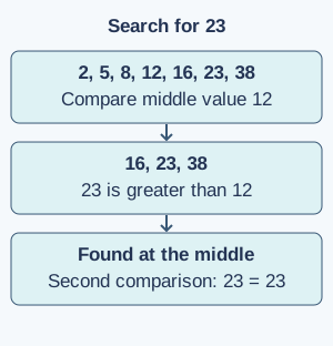
A binary-search example — For the sorted list [2, 5, 8, 12, 16, 23, 38], target 23 is above the middle value 12, so retain [16, 23, 38]. Its middle is 23, so the target is found after two comparisons. Target 15 would narrow to a range with no matching value. Keeping a record of bounds avoids revisiting a discarded half.Sorted values allow the range to narrow: compare 12, retain 16, 23 and 38, then find 23. This example takes two value comparisons. Full-size diagram
Comparing searches — Compare algorithms using the same task and dataset, considering number of comparisons, preparation and assumptions. Binary search can use far fewer comparisons on a large sorted list, but sorting a small unsorted list for one search may cost more work than a linear search. 'Faster' needs a defined measure; hardware timings alone can mix algorithm effects with other factors.
Bubble sort — A simple bubble sort compares neighbouring items and swaps them when they are out of order, repeating passes until sorted. One left-to-right pass through [4, 1, 3] produces [1, 3, 4]. Longer lists may need several passes. A version can stop early when a whole pass makes no swaps; merely performing one pass does not sort every list.
Insertion sort — Insertion sort builds a sorted part at the beginning of a list, called a sorted prefix. Place each next item into the correct position in that part, moving larger items along. Starting with [4], insert 1 to make [1, 4], then insert 3 to make [1, 3, 4]. This can be useful for nearly sorted lists. Show each step, not just the final answer.
Sorting choices — Bubble and insertion sort can produce the same order with different amounts of work. Try sorted, reverse-sorted and mixed lists, counting the same kind of operation, such as comparisons, for both methods. When sorting surnames, decide how ties and case, capital versus lower-case letters, are treated. The best choice depends on input size, starting order and what the task needs.
Reasoning and testing
Correctness and edge cases — A correct algorithm meets its defined requirements for all allowed inputs, not just the example used to design it. Consider an empty list, one item, repeated values and a missing target when testing a search. State what each case should produce before running it. Passing several tests increases confidence but is not by itself proof for every possible input.
Efficiency and usefulness — A useful solution balances correctness, work required, memory, clarity and the needs of users. A more elaborate method is not automatically better for a small task. Explain the assumptions behind a recommendation and distinguish counting algorithm steps from measuring a particular computer's running time. A fast wrong answer remains wrong.
Refining a solution — Use evidence from traces, tests and feedback to improve the algorithm or its model. Change one identified cause, then rerun relevant tests, including ones that passed before. Record why the change works and what limits remain. Repeatedly changing code at random without checking a prediction makes it difficult to learn which change fixed the problem.
Test yourself
50 questions · Random sets of 10. These quick checks support revision; practise longer explanations and justified judgements too.
Mind map
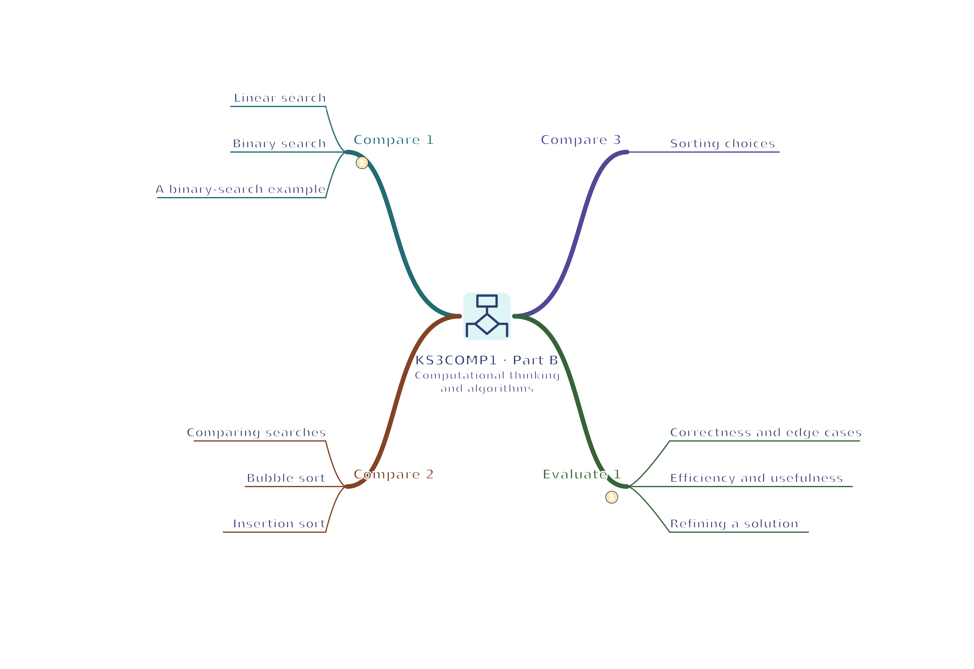
Use the branches to recall the ideas and explain their connections. Check the revision notes for the full detail.
KS3COMP1 · 1
View KS3COMP1 · 1 mind mapOpen the full-size map to zoom. Use the printable view for A4 landscape or enlarge to A3.
 Mr Kidman's Classroom