Probability scale — Probability lies from 0 for impossible to 1 for certain. A probability of 0.5 means equally likely to occur or not occur in the model, not that every pair of trials contains exactly one success.
Equally likely outcomes — For a fair six-sided die each face has probability 1/6, so P(even) = 3/6 = 1/2. Favourable outcomes are the results you want to count; elementary outcomes are the separate basic results, here the six faces. Dividing the number of favourable outcomes by the total number works when those basic outcomes are equally likely.
Unequal likelihood — A spinner's sectors may have unequal angles: a 90° red sector has probability 90/360 = 1/4 in an ideal uniform spinner model. Counting sector labels alone fails if sector sizes differ.
All outcomes — Outcomes are mutually exclusive if they cannot happen together in one trial. If they also cover every possible result, their probabilities sum to 1. If red, blue and green are the only results with probabilities 0.2, 0.5 and p, then p = 0.3. Overlapping events cannot simply be added.
Complement — The probability an event does not happen is 1 − P(event). If P(rain) = 0.35, P(no rain) = 0.65 in the same model. These two events cover every possibility without overlap.
Experiments
Frequency and relative frequency — If a spinner lands red 18 times in 60 spins, relative frequency is 18/60 = 0.3. This estimates the probability; it need not equal the theoretical value or the next trial's result.
Randomness and fairness — Random means an individual outcome is uncertain; fair means the model gives the stated outcomes equal chances. A biased die can still be random. Keep the method consistent and record every trial.
Larger trials — Independent trials are trials where one result does not change the probabilities for the next. With many such trials and unchanged conditions, relative frequencies tend to settle near the underlying probabilities, but fluctuations remain. A small trial difference is not proof of bias; a long consistent discrepancy deserves investigation.
Expected frequency — If P(success) = 0.3, 200 trials have expected frequency 200 × 0.3 = 60. This is a model expectation, not a guaranteed count. Real outcomes vary.
Sets and enumeration
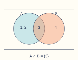
Set notation — A set lists distinct elements. For A = {1,2,3} and B = {3,4}, intersection A ∩ B = {3}; union A ∪ B = {1,2,3,4}. A union includes overlap once.Union and intersection. Original illustrative model. Full-size diagram
Venn diagrams — Place items in the overlap first, then in the exclusive regions and outside both inside the universal-set rectangle. If A has 12 members and 5 are also in B, the A-only region has 7.
Systematic lists — For tops R,B and trousers S,L, list RS, RL, BS, BL. A table with one choice along each axis prevents omissions. Different basic outcomes can give the same calculated result. For example, on two dice (1,3) and (2,2) are different outcomes even though both sums are 4.
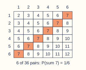
Two dice sample space — A 6 by 6 grid gives 36 ordered pairs for two independent fair dice. Sum 7 has six pairs, so probability is 6/36 = 1/6; sum 2 has only (1,1), so 1/36. The eleven possible sums are not equally likely.Two fair dice sample space. Original illustrative model. Full-size diagram
Combined coin outcomes — Two independent fair coin tosses have HH, HT, TH, TT, each probability 1/4. Exactly one head has two outcomes, probability 1/2. Order distinguishes HT from TH.
Without replacement — Drawing two labelled counters without replacement excludes choosing the same counter twice. A sample space lists all possible outcomes. With labelled counters A, B and C, the ordered outcomes without replacement are AB, AC, BA, BC, CA and CB. AA, BB and CC are impossible because the first counter is not returned. State whether order matters and whether items are returned. Do not reuse an independent-draw model without checking.
Conclusions
Probability arguments — If a fair die lands on six five times in a row, the probability of six on the next independent roll is still 1/6. It is neither less likely because six has just occurred nor more likely because another result is “due”. Explain using unchanged next-trial probabilities; apparent streaks do not alter the mechanism.
Limitations — A theoretical model assumes a mechanism and probabilities. Compare it with experimental data, consider sample size and method, and explain uncertainty instead of claiming a small experiment proves fairness.
Test yourself
50 questions · Random sets of 10. These quick checks support revision; practise longer explanations and justified judgements too.
Mind map
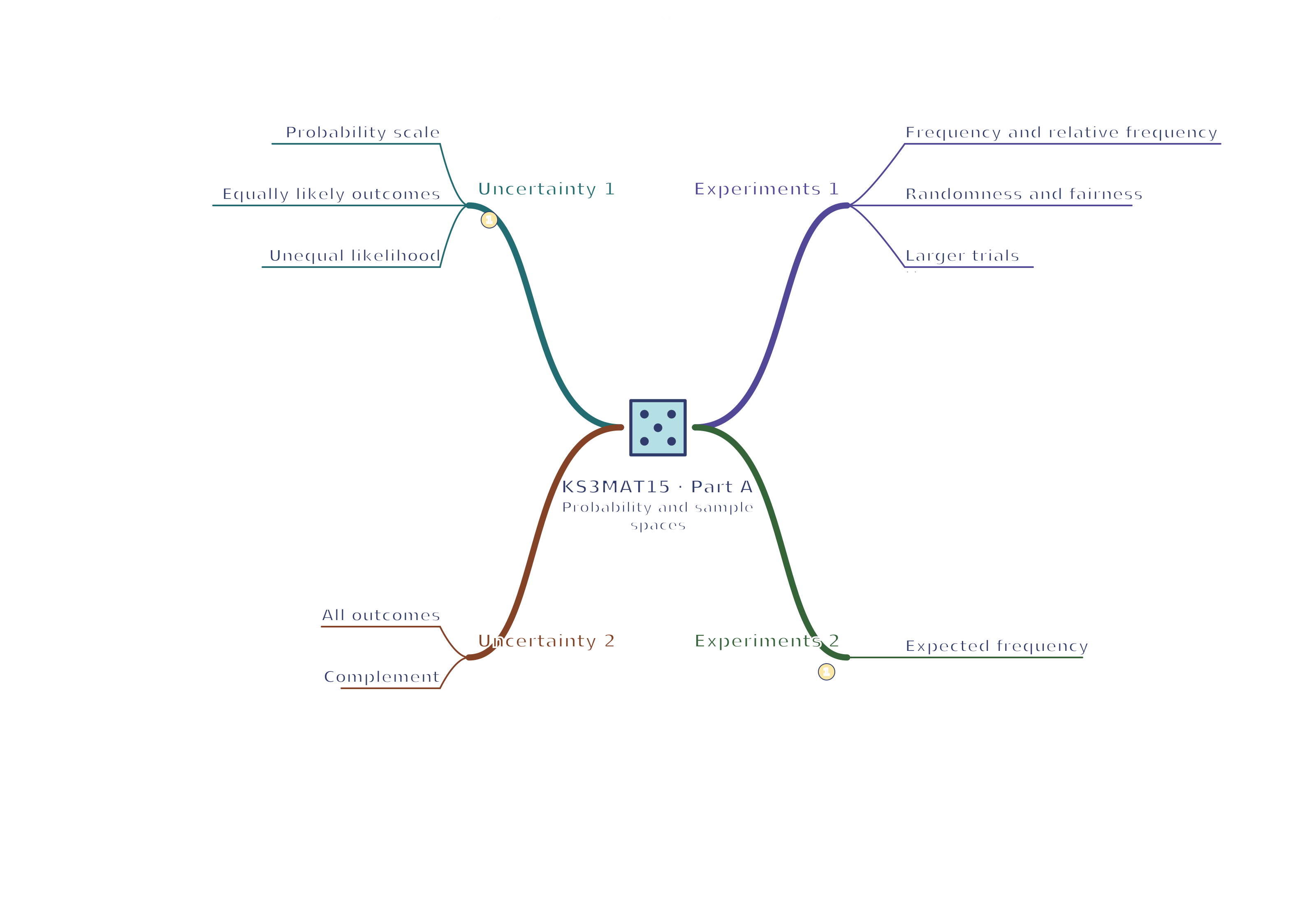
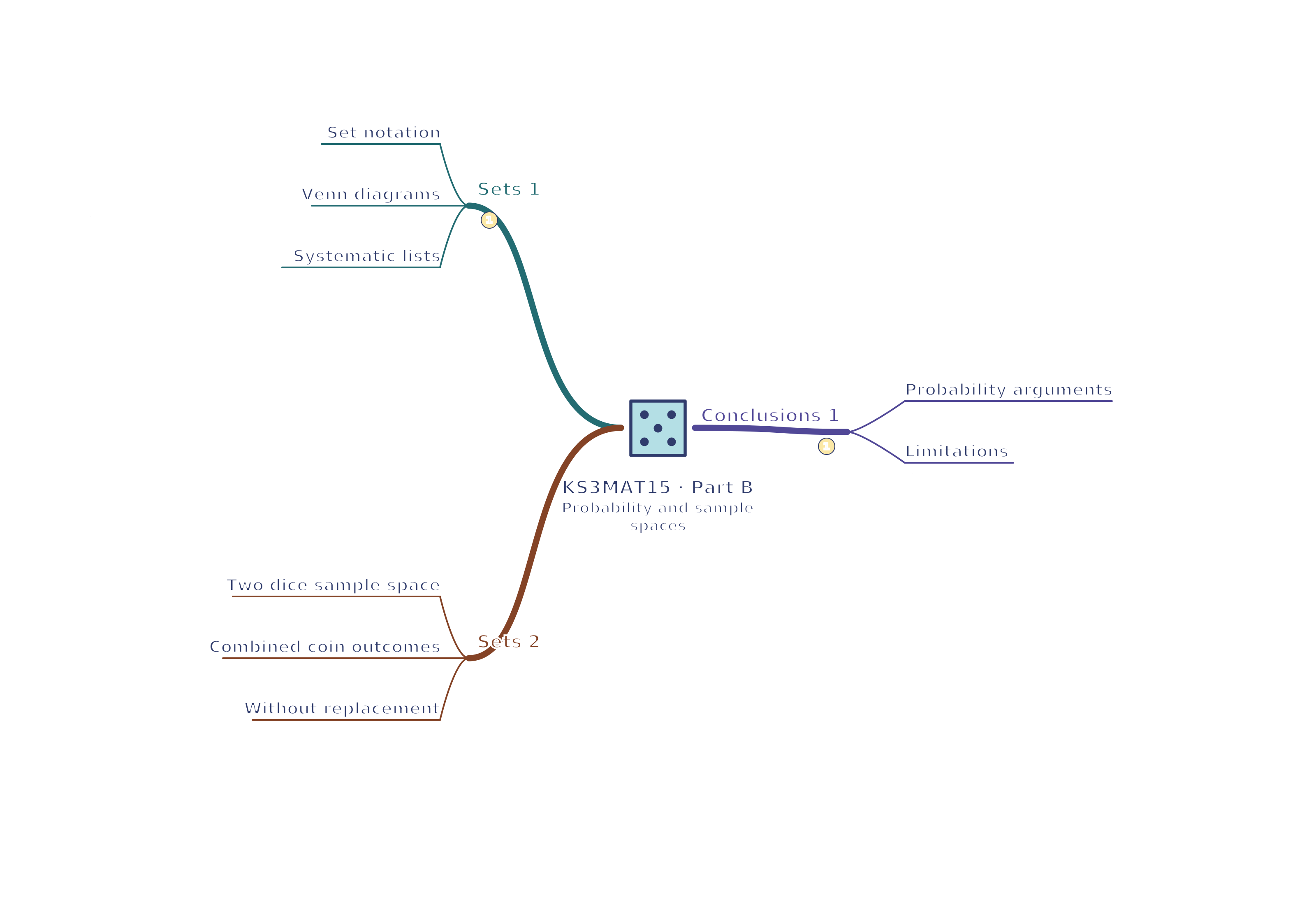
Use the branches to recall the ideas and explain their connections. Check the revision notes for the full detail.
KS3MAT15 · 1
View KS3MAT15 · 1 mind mapOpen the full-size map to zoom. Use the printable view for A4 landscape or enlarge to A3.
 Mr Kidman's Classroom