Owners' savings — An owner can invest personal savings to fund a start-up or expansion. This avoids a scheduled loan repayment but sacrifices the owner's next best use of the money and concentrates personal risk. The amount available may be too small for the proposed scale; finance with no interest is not finance with no opportunity cost.
Retained profit — Retained profit is profit kept within a business rather than distributed to owners. It can support investment without issuing more shares or taking another loan, but a start-up has no past retained profit and owners may prefer a distribution. Accumulated accounting profit is not necessarily an equally large cash balance available today.
Selling assets — Selling a surplus vehicle, building or investment can release cash. Assess the sale proceeds, speed and effect on future operations: selling an essential machine may reduce output or require costly replacement. A sale-and-leaseback releases capital while creating continuing rental commitments; the resource is no longer owned.
External sources and methods of finance
Sources versus methods — A source identifies who provides finance, while a method identifies the arrangement. A bank might provide a loan or overdraft; an angel might buy shares. Compare amount, duration, cost, security, repayment flexibility and control rather than treating all external money as one interchangeable source.
Loans and interest — A loan provides an agreed sum with contractual repayment and interest terms. It can match a long-lived investment, allowing costs to be spread over time, but repayments continue if sales disappoint. Security requirements and variable interest can increase risk. Compare total cost and cash timings, not only the advertised interest percentage.
Overdrafts — An overdraft permits a current account to become negative up to an agreed limit. It can bridge short timing gaps and interest normally applies to the amount used, but fees, changing terms and possible withdrawal make it a fragile permanent funding source. A continuously growing overdraft may indicate a structural cash problem.
Trade credit — Trade credit allows a business to receive inputs before paying its supplier. It can help match payments to receipts, but missed deadlines can damage supply relationships and creditworthiness; early-payment discounts may be forgone. It delays a cash outflow rather than removing the cost of the inputs.
Leasing — Leasing gives use of an asset in exchange for periodic payments rather than an initial purchase. It can preserve cash and provide access to modern equipment, although total payments and contractual restrictions may be substantial. Maintenance responsibility and end-of-term rights depend on the agreement, so do not assume automatic ownership.
Share capital — Issuing shares raises owners' funds without the fixed repayment schedule of a loan. New owners may expect influence and returns, and existing shareholders' percentage holdings can be diluted. A private company cannot simply sell shares to the general public in the same way as a public company meeting the relevant requirements.
Angels and venture capital — Business angels invest their own money and may contribute expertise; venture-capital organisations invest funds in ventures with substantial growth potential. Both can demand ownership, influence and an eventual exit. A business with modest predictable returns may be unsuitable even if it would be a sound small enterprise.
Peer-to-peer and crowdfunding — Peer-to-peer lending connects borrowers and lenders through a platform; crowdfunding collects contributions from many supporters. A campaign can involve loans, equity, rewards or donations, with different obligations. Public attention does not guarantee enough finance, and campaign costs, disclosure and fulfilment promises require planning.
Family, other businesses and grants — Family or friends may offer flexible funds, but ambiguous terms can damage relationships. Another business may invest for strategic reasons that reduce independence. A grant may not need repayment if conditions are met, yet eligibility, timing, permitted uses and monitoring can constrain it. Do not assume grants are universally available or unrestricted.
Matching finance to the need — A seasonal stock purchase and a ten-year production asset create different funding needs. Compare a short working-capital facility with longer-term funds, using forecast cash flows and a downside scenario. The cheapest nominal rate may be inferior if repayment falls before customer receipts or control conditions obstruct the strategy.
Liability and financing choices
Unlimited liability — In an ordinary sole trader or partnership model, business debts can expose owners' personal assets. This may discourage large borrowing or risk-taking even where a lender is willing to lend. Partners' agreements and the exact legal form matter; do not classify every organisation containing the word partnership identically.
Limited liability and its limits — A company's owners generally limit their exposure to the amount invested, encouraging pooled investment. The company itself still owes its debts; limited liability does not guarantee loan approval or prevent failure. Personal guarantees or misconduct can change an individual's exposure, so distinguish the general business principle from specific legal advice.
Form and access to funds — An unincorporated sole trader cannot issue company shares. A limited company may offer equity to suitable investors, although the actual ability to raise funds depends on performance, plans, credibility and investor demand. Banks consider repayment prospects as well as organisational form; incorporation alone does not create financial strength.
Business plans and cash-flow forecasting
A coherent business plan — A useful plan connects objectives, researched demand, marketing, staffing, operations and finance. Lenders need credible repayment evidence, while equity investors also consider growth and control. Explain assumptions and contingencies: attractive presentation cannot repair incompatible sales, capacity and cash forecasts.
Cash inflows and outflows — A cash-flow forecast records expected receipts and payments in the periods when cash moves. Customer receipts may occur after a credit sale, and buying a machine creates a cash payment even though its full cost is not treated as one year's operating expense. Include relevant finance receipts and repayments without calling them sales revenue.
Net and closing cash — Net cash flow = total cash inflows − total cash outflows. Closing balance = opening balance + net cash flow; the closing balance becomes the next period's opening balance. A negative net flow means cash fell during the period, whereas a negative closing balance means the forecast account is overdrawn under this model.
Worked cash forecast — A fictional firm opens April with £6000, receives £18000 and pays £22000. Net cash flow is −£4000 and the closing balance is £2000, not an overdraft. If May's net flow is −£3500, its closing balance becomes −£1500, so a funding or operational response is needed before that shortage occurs.
Changing assumptions — Model changed payment dates, sales volumes, input costs or finance rather than merely altering the final balance. Delaying a £4000 supplier payment from April to May improves April's closing cash by £4000 but worsens May's net flow by the same amount. Unless another change occurs, it does not create £4000 of profit.
Forecast use and limitations — A forecast supports early borrowing discussions, collection policies and timing decisions. Its reliability depends on customer payment behaviour, demand, cost estimates and shocks. Compare alternative scenarios and update actual results; a detailed spreadsheet does not turn uncertain assumptions into facts or certify a viable business.
Sales forecasting and uncertainty
Purpose of a sales forecast — A sales forecast estimates future volume or value over a stated period. It informs capacity, staffing, stock, marketing and cash planning. Use a common period and product definition so the operations plan can fulfil the forecast and the finance plan can fund it; an aspirational target is not automatically an evidence-based forecast.
Factors affecting forecasts — Customer tastes, population, incomes and economic conditions affect demand, while rivals' prices, launches and capacity can change a firm's share. Distinguish market growth from the business's own sales growth. Use both relevant research and past patterns, explaining why past conditions may or may not persist.
Forecast difficulties — New products lack a direct sales history; short records may confuse seasonal fluctuations with a trend. Competitors and external shocks can invalidate an otherwise sensible projection. Present ranges or scenarios where appropriate and explain consequences of overestimating and underestimating rather than pretending either error is costless.
Sales revenue and cost behaviour
Volume and value — Sales volume counts units sold; sales revenue measures their monetary value. For a single uniform price, revenue = price × volume. At £25 for 800 units, revenue is £20000. With several products or discounts, calculate each relevant price-volume combination before adding; multiplying an unweighted average price can mislead.
Fixed costs — Fixed costs do not change with output within the stated period and relevant range, such as an agreed factory rent. Fixed does not mean unchanged forever: a larger site, revised contract or extra capacity can create a step increase. A monthly fixed cost must not be compared with annual revenue without converting periods.
Variable costs — Variable costs change with output in the stated model. Total variable cost = variable cost per unit × output when the unit rate is constant. At £9 per unit and 800 units, total variable cost is £7200. Bulk discounts, overtime or waste can break the assumption of a constant rate.
Total and average costs — Total cost = fixed cost + total variable cost. Average total cost = total cost ÷ output, for positive output. If fixed cost is £4800 and variable cost £9 for 800 units, total cost is £12000 and average cost £15. Spreading fixed costs can reduce average cost without reducing the total fixed bill.
Costs and decision context — Classify costs according to their behaviour in the scenario, not their everyday name. Labour may be salaried, piece-rate or overtime; electricity may combine a standing charge and usage. A change can reduce one cost while increasing another, so assess the relevant total and any quality or capacity consequences.
Contribution, break-even and margin of safety
Contribution per unit — Contribution per unit = selling price − variable cost per unit. It contributes towards fixed costs first and then profit. A fictional £25 product with £9 variable cost contributes £16 per unit; this is not £16 profit per unit while fixed costs remain uncovered.
Break-even calculation — Break-even output = total fixed costs ÷ contribution per unit, assuming positive contribution and a consistent period. With £4800 fixed costs and £16 contribution, break-even is 300 units. A fractional result normally requires rounding up to the next whole sale when indivisible units must cover all costs.
Total contribution and profit — Total contribution = contribution per unit × units sold. Profit in this simplified model = total contribution − fixed costs. At 800 units, contribution is £12800 and profit £8000. Reconcile this with revenue £20000 less total costs £12000 to check the calculation.
Margin of safety — Margin of safety = actual or forecast sales volume − break-even volume. With 800 forecast sales and 300 break-even, it is 500 units. A percentage margin uses a stated denominator, commonly forecast sales: 500 ÷ 800 × 100 = 62.5%. It measures sales headroom under the assumptions, not guaranteed protection against shocks.
Reading a break-even chart — Output belongs on the horizontal axis and costs/revenue on the vertical axis for a stated period. Total revenue begins at zero in the simple uniform-price model; total cost begins at fixed cost. Their intersection marks break-even, the revenue-above-cost region profit and the reverse region loss. Read scales and units carefully.Worked straight-line model with price £25, variable cost £9 per unit and fixed cost £4800. Teal revenue and orange total cost intersect at 300 units and £7500. Q means units sold in the same period; the graph ends at 1000 units.
Changing the model — A higher fixed cost shifts the total-cost line upward and normally raises break-even. A higher variable cost steepens total cost and reduces contribution; a higher price steepens revenue but may also reduce demand. Calculate the changed break-even and compare achievable sales rather than declaring a price increase automatically beneficial.
Limitations of break-even — Straight lines assume constant price and variable cost per unit, constant fixed cost in the relevant range, and output sold. Multi-product sales mixes, capacity limits, stock changes and uncertainty complicate the model. A break-even chart does not show payment dates, so an apparently profitable operation can still face a cash shortage.
Budgets and variance analysis
Budgets as plans — A budget sets a financial plan or target for a stated period, such as sales revenue or departmental spending. It supports coordination, responsibility and control. A forecast estimates what may happen; a budget can reflect what management intends, although both need credible assumptions and suitable revision when circumstances change.
Historical and zero-based approaches — A historical budget adjusts previous figures, making preparation quicker but possibly preserving waste or outdated activities. Zero-based budgeting requires proposed spending to be justified afresh, encouraging challenge but using management time and difficult judgements. Neither method eliminates uncertainty or guarantees that all departments reveal honest estimates.
Interpreting variances — A variance compares actual with budgeted performance using a clearly stated sign convention. Spending £46000 against a £50000 cost budget is £4000 favourable on cost; revenue £46000 against a £50000 revenue budget is £4000 adverse. Favourable means favourable against that measure, not proof that the underlying decision benefited the business.
Investigating causes — Lower training spending might explain a favourable cost variance but later reduce quality. Higher material spending may accompany higher profitable sales rather than inefficiency. Separate price, quantity and context where evidence permits, then decide whether to correct action, revise assumptions or accept a justified deviation.
Behaviour and budgeting — Unrealistic budgets can demotivate or encourage short-term manipulation. Managers may build slack into requests or spend remaining allocations to protect next year's funding. Participation and meaningful performance measures can help, but budget control should still consider strategy, quality and changing conditions rather than one isolated financial target.
Profit measures and profitability
Gross profit — Gross profit = sales revenue − cost of sales. It shows the amount remaining after the direct cost of the goods or services sold before the stated operating expenses. Cost of sales is not automatically identical to cash paid for inventory in the period; use the figures and classifications supplied.
Operating profit — Operating profit = gross profit − other operating expenses in the simplified income statement used here. It reflects the core operation before the stated finance costs and tax. When an extract has extra operating income or a different presentation, follow its labels and avoid deducting an expense twice.
Profit for the year — Profit for the year, often called net profit in this course, is the profit remaining after the stated finance costs and tax. For revenue £200000, cost of sales £110000 and operating expenses £50000, gross profit is £90000 and operating profit £40000. Deducting £4000 interest and £6000 tax leaves £30000. The specification appendix uses a simplified layout deducting interest without a separate tax line; follow the actual supplied extract and do not invent an extra tax deduction.
Profit margins — Gross margin = gross profit ÷ revenue × 100; operating margin and profit-for-year margin use their corresponding profit numerator. The example produces 45%, 20% and 15%. State the measure: a business can increase sales and absolute profit while a margin falls, so the two observations are not contradictory.
Improving profitability — A higher price, better sales mix, lower waste or more efficient resource use may improve margins, but each depends on demand and implementation. Cutting service or training can damage future revenue. Compare the size and timing of expected benefits with costs and rival responses rather than listing cost cutting as universally effective.
Profit versus cash — A credit sale can contribute to profit before the customer pays; a loan receipt increases cash without being sales profit. Purchasing a long-lived asset uses cash, while depreciation allocates its cost over time in accounts. A profitable growing business can therefore run out of cash if receipts lag payments.
Liquidity, financial position and working capital
Financial-position categories — A statement of financial position records assets (resources the business controls), liabilities (obligations it owes) and equity (the owners' residual interest after liabilities are deducted from assets) at a date rather than income over a period. Current assets include inventory, receivables and cash expected to be realised in the operating cycle or short term; current liabilities include relevant short-term obligations. Use the extract's classifications and date consistently.
Working capital — Working capital = current assets − current liabilities. With current assets £70000 and current liabilities £40000, working capital is £30000. Positive working capital is not the same as £30000 cash: some assets may be unsold stock or unpaid customer balances, while liabilities may fall due before they turn into receipts.
Current ratio — Current ratio = current assets ÷ current liabilities, expressed as x:1. The example gives 1.75:1. A ratio above one does not guarantee every bill can be paid on time, and a high ratio may reflect slow-moving stock or unproductive cash. Interpret it against sector, trading cycle and trends rather than a universal ideal.
Acid test ratio — Acid test = (current assets − inventory) ÷ current liabilities. If inventory is £30000, the example gives 1:1. It excludes stock because sale and collection may take time, but receivables may also be late or irrecoverable. A low figure deserves investigation rather than automatic failure prediction.
Managing liquidity — Faster collection, appropriate inventory reduction, agreed supplier terms and suitable long-term finance can release pressure. Aggressive collection may lose customers; low stock can cause shortages; late supplier payment can disrupt deliveries. Selling fixed assets or taking a loan may help cash immediately while changing future capacity, interest and repayment commitments.
Cash discipline and growth — Rapid expansion can absorb cash in stock, receivables and operating costs before receipts arrive. Coordinate credit control, purchasing, investment and funding rather than relying on a favourable annual profit forecast. A rolling cash forecast and realistic downside scenario reveal timing risks that balance-sheet ratios alone cannot show.
Causes and processes of business failure
Internal causes — Weak cash control, unsuitable borrowing, poor products, inconsistent quality, excessive costs and ineffective leadership can threaten survival. Explain a causal sequence: unreliable deliveries can lose customers, reduce receipts and leave fixed obligations unpaid. An accounting loss and an inability to pay a bill are related risks but not identical events.
External causes — A recession, input-price shock, disruptive competitor or supply interruption can undermine even a previously successful firm. Exposure differs with sector, customer base, finance and alternatives. Distinguish the trigger from vulnerabilities such as dependence on one supplier; avoid asserting one universal cause from an isolated statistic.
Interacting warning signs — Falling margins, overdue receivables, rising debt and repeated quality complaints may reinforce one another. A cash rescue alone may postpone failure if demand or operations remain unsustainable. Evaluate recovery options using both financial and non-financial evidence, including feasibility, time and stakeholder effects.
Production methods, productivity and efficiency
Job production — Job production makes a distinct item or project for a customer's requirements, such as a fictional bespoke stage set. It can support customisation and skilled work but may involve higher unit costs, complex scheduling and dependence on specialist staff. High price is useful only if customers value the difference enough to cover costs.
Batch production — Batch production makes a group of similar items before switching to another group. It offers variety and some repetition economies, but changeovers, waiting and work-in-progress stock can add cost. Appropriate batch size depends on demand, setup time, storage and the risk of unsold output.
Flow production — Flow production moves standardised output through a continuous sequence of tasks. High sustained volume can spread setup costs and support consistency, but machinery, inflexibility and a bottleneck or breakdown can be expensive. It is not automatically appropriate for low-volume or highly varied demand.
Cell production — Cell production organises a team and equipment around a product or process family. It can combine teamwork, flexibility and reduced movement, though reorganisation and multi-skilling require investment. Evaluate fit to product variety, layout and skills rather than treating every team as a production cell.
Productivity calculations — Labour productivity = output ÷ labour input for the stated period, such as units per worker per week or units per worker-hour. If 12 workers make 1800 units in a week, output is 150 units per worker-week. Use consistent hours and quality: a higher count of defective units is not necessarily an improvement.
Productivity and competitiveness — Training, motivation, equipment, process design and reliable inputs can increase output per input. Lower unit labour cost may allow lower prices or higher margins, but investment cost and demand matter. Productivity measures a ratio; production measures total output, so output can grow merely because more workers are used.
Efficiency and input intensity — Efficiency concerns using resources effectively, with minimum average cost in the course's production model. A capital-intensive process relies relatively heavily on equipment; a labour-intensive process relies relatively heavily on people. Compare scale, finance, skills, flexibility and service quality: minimum wage cost alone does not establish minimum total cost.
Capacity utilisation
Calculating utilisation — Capacity utilisation = actual output ÷ maximum possible output × 100 for comparable conditions and periods. Output of 7200 units against 9000 capacity gives 80%, leaving 1800 units of measured spare capacity. Define realistic capacity consistently; a temporary overtime maximum is different from sustainable normal capacity.
Under-utilisation — Spare capacity spreads fixed costs over fewer units and may signal weak demand, seasonality or an intentionally retained buffer. It can also permit rapid response and maintenance. A low rate is therefore a prompt to investigate causes and financial effects, not evidence that all spare resources should immediately be removed.
Very high utilisation — A plant close to maximum output may spread fixed costs well but have little flexibility for demand peaks or breakdowns. Overtime, rushed work and deferred maintenance can raise cost and reduce quality. Output above a quoted normal capacity can indicate temporary exceptional working or a definition issue rather than a physically impossible percentage.
Managing utilisation — Increase suitable demand, share resources, subcontract peak work or adjust capacity, depending on the cause. Closing capacity can improve the percentage while reducing total potential sales; promotion can increase output while reducing contribution. Evaluate financial and operational consequences together rather than optimising the percentage alone.
Inventory control, lean production and waste
Why hold stock — Inventory can include raw materials, work in progress and finished goods. It buffers uncertain demand and delivery, supports production continuity and may secure purchasing discounts. Holding it ties up working capital and incurs storage, insurance, damage, obsolescence and waste costs; no single stock level suits every product.
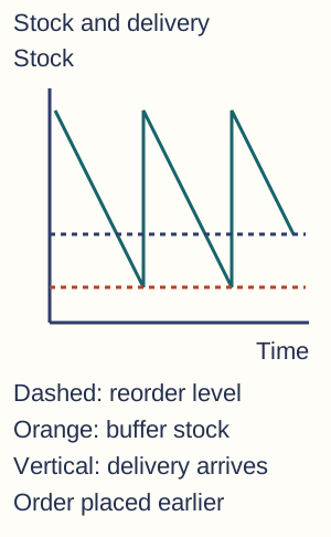
Reading a stock-control diagram — Time is on the horizontal axis and stock quantity on the vertical axis. Stock falls as units are used and rises when a delivery arrives. The reorder level is the stock amount that triggers a new order; the reorder quantity is the amount ordered. Lead time is the delay between ordering and receiving goods, and buffer stock is the reserve held against unexpected demand or delay. Reaching the reorder level triggers an order; it is not the same event as receiving that order.Schematic steady stock use and discrete deliveries, not measured data. The upper dashed line triggers an order; the delivery arrives later, shown by a vertical jump. The orange dashed buffer is retained in this undisturbed illustration.
Reorder and buffer calculations — In a simplified steady-use model, reorder level = expected use during lead time + buffer. At 40 units daily and a three-day lead time, a 30-unit buffer gives a reorder level of 150 units. Buffer protects against some variation but cannot guarantee continuity through every possible delay or demand surge.
Poor stock control — Insufficient stock can halt production or lose customer orders, while excess stock raises cost and masks process problems. Inaccurate records can produce both shortages and surpluses in different items. Consider forecast quality, supplier reliability and traceability rather than assuming a larger warehouse solves the underlying issue.
Just-in-time — Just-in-time aims to receive or produce what is required close to when it is needed, reducing inventory and exposing process problems. Reliable suppliers, short lead times, coordinated information and quality at source matter. Minimal buffers can increase vulnerability to disruptions; JIT is an operating system, not merely deciding never to hold stock.
Lean production and waste — Lean approaches seek customer value with fewer wasted resources, such as unnecessary movement, waiting, defects and overproduction. Process mapping, worker involvement and reliable flow can improve lead times and costs. Cutting resources indiscriminately can damage resilience or service and should not be confused with removing non-value-adding activity.
Quality management and continuous improvement
Quality and fitness for purpose — Quality concerns meeting agreed customer requirements consistently, not necessarily using the most expensive design. Specify measurable standards relevant to the segment, such as reliability, safe operation, delivery accuracy or response time. A luxury feature that customers do not want can add cost without improving fitness for purpose.
Quality control — Quality control checks outputs against standards and identifies defects, often through inspection or sampling. It can stop unsuitable products reaching customers, but discovering defects late wastes resources and may not reveal the cause. A sample cannot prove every untested item is faultless; inspection must use appropriate measures and procedures.
Quality assurance — Quality assurance builds agreed processes and responsibilities intended to prevent defects throughout production or service delivery. Training, specifications, records and supplier standards support it. It reduces reliance on final inspection but requires consistent implementation and review; writing a procedure does not ensure staff can or do follow it.
Circles and total quality — Quality circles bring employees together to investigate and propose improvements. Total Quality Management treats quality as an organisation-wide responsibility involving customer focus, staff and suppliers. Suggestions need resources, management support and evidence; neither a meeting nor a slogan guarantees a measurable improvement.
Kaizen and improvement — Kaizen emphasises continuing incremental improvement with employee involvement. Small changes to layout or task sequence can accumulate into savings and fewer errors, but time, training and participation have costs. Measure before-and-after performance and check that an apparent local gain does not move a problem elsewhere.
Competitive effects — Consistent quality can reduce rework, refunds and reputational damage while supporting repeat purchases and differentiation. The benefit depends on the cost of prevention and customers' response. Compare quality costs across the whole operation rather than treating the inspection department's budget as the only expense.
Economic conditions and business decisions
Inflation and price indices — Inflation is a rise in the general price level, measured here using changes in a consumer-price index. An index rising from 120 to 126 represents (126 − 120) ÷ 120 × 100 = 5% inflation. The rise is six index points; percentage growth uses the original index value as its denominator. A lower positive inflation rate means prices are rising more slowly, not generally falling; one input's price can move differently from the average.
Business effects of inflation — Input and wage pressures can squeeze margins if selling prices cannot rise; changing prices and uncertainty add planning costs. Some firms can protect margins through differentiation or contracts while others cannot. Compare nominal sales growth with price changes before interpreting it as higher real output or improved competitiveness.
Exchange-rate quotation — An exchange rate states how much of one currency exchanges for another. If £1 buys $1.20 and later $1.35, sterling has appreciated against the dollar. A $270 imported item changes from £225 to £200 before other costs. Always identify the quote direction before applying the words appreciation or depreciation.
Exchange rates and trading — A stronger home currency can make foreign-currency imports cheaper in home money while making a fixed home-currency export price dearer for foreign buyers. Effects depend on invoicing, contracts, imported components, demand elasticity and rival action. A firm that both imports and exports may face offsetting effects rather than a single automatic gain or loss.
Interest rates — Higher borrowing rates increase the cost of variable-rate debt and new finance, potentially discouraging investment. Consumer demand for credit-sensitive products may weaken, while savers can receive more interest. Fixed-rate contracts, debt exposure and cash holdings affect timing and magnitude; every business is not affected equally.
Tax and public spending — Higher taxes on income or spending can alter customers' disposable income and demand; taxes on profits or inputs affect retained funds and costs. Government spending can create demand for suppliers and improve infrastructure. Explain the particular channel and affected customers rather than assuming all taxes or spending have identical effects.
Business cycle — Expansion and downturn describe changes in overall economic activity, with consequences for sales, employment and confidence. Cyclical luxury or investment-goods businesses may be more exposed than essential services, but individual performance also depends on strategy and local conditions. A national downturn does not imply every firm's revenue must fall.
Uncertainty and response — Uncertain demand, rates or policy may lead a firm to postpone investment, retain liquidity or use flexible capacity. These responses have opportunity costs if growth arrives sooner than expected. Use scenarios and identify which assumptions would reverse a decision; do not present a hypothetical macroeconomic scenario as a current economic fact.
Legal influences on operations
Consumer and employee protection — Rules protecting customers and workers can affect product information, quality, contracts, working arrangements and training. Compliance can raise some costs while improving trust, retention and competition on standards. These notes explain business effects rather than provide a definitive legal checklist; apply the facts and rules supplied in an examination scenario.
Environmental protection — Environmental requirements can change waste handling, emissions, materials and investment choices. Compliance or cleaner technology may raise initial expenditure but reduce resource use or support reputation. Evaluate the size and timing of costs and benefits, and who bears or receives them, including effects across suppliers rather than assuming a green claim proves a net environmental gain.
Competition and safety — Competition policy can constrain anti-competitive conduct or acquisitions, while health-and-safety requirements affect equipment, processes and staff preparation. They can protect stakeholders and encourage fairer markets as well as impose compliance costs. Distinguish a general business mechanism from asserting that a particular real action is legally permitted or prohibited.
Competitive environment and connected decisions
Competition and market size — More or stronger rivals can pressure prices, increase promotion costs and stimulate innovation, but may also expand customer awareness of a category. A growing market can support entrants while still reducing an incumbent's share. Assess differentiation, entry barriers and market growth alongside the simple count of competitors.
Responding across functions — A price response affects contribution and break-even; a product redesign affects operations, training and cash; an expansion changes funding and capacity. Develop a recommendation through these connected effects using fictional data and explicit assumptions. A convincing judgement identifies a feasible action, its main risk and the condition under which another option becomes preferable.
Test yourself
50 questions · Random sets of 10. These quick checks support revision; practise longer explanations and justified judgements too.
 Mr Kidman's Classroom