 Mr Kidman's Classroom


Revise the key ideas
Likelihood and experimental evidence
- Probability scale — Probability lies between 0 and 1: 0 is impossible, 1 certain and 0.5 an even chance. Convert consistently between fractions, decimals and percentages. Likely does not mean guaranteed; a single outcome cannot show whether an assigned probability was correct.
- Theoretical models — Count favourable outcomes / all outcomes only when outcomes are equally likely. A fair six-sided die gives P(even)=3/6=1/2. A biased spinner's labelled sections may not have equal probabilities, so counting labels alone is insufficient.
Favourable outcomes are the ones matching the event you are counting; the word does not necessarily mean desirable.
- Complement — An event and its complement exhaust the possibilities without overlap, so P(not A)=1−P(A). If probability of a late bus is 0.18, probability of not late is 0.82. Define the event carefully: not winning can include both drawing and losing.
- Relative frequency — Estimate probability as observed event count / trial count. If 28 of 80 deliveries are late, estimated probability is 0.35. Keep a consistent event definition and report the number of trials; observed proportions vary between samples.
- Expected frequency — Multiply probability by the number of trials: E=np. With p=0.3 in 200 trials expect 60 events on average. An expectation is not a guaranteed realised count, and it need not be a whole number when describing the average of many repeated trials.
In E = np, E is expected frequency, n is the number of trials and p is the probability of the event.
- Long-run behaviour — Under suitable random repeated trials with a stable probability, relative frequency tends to settle nearer that probability as trial count grows. It does not move closer after every extra trial, and past failures do not make an independent future success compulsory.
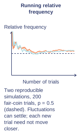
- Assess possible bias — Compare observed counts with expected values, taking trial size and ordinary variation into account. A die showing six twice in twelve rolls is compatible with many models; a large, lasting difference across many trials is stronger reason to question fairness or collection. Formal significance tests are not required.
- Simulation — Use random digits or calculator outcomes with probabilities matching the model. To simulate probability 0.3 using equally likely digits 0–9, designate three digits as success. State independence assumptions and run enough repetitions; a poor mapping biases the simulation before it begins.
Absolute and relative risk
- Absolute risk — Risk is a probability of a specified outcome in a defined group and period. If 4 of 200 items fail, absolute risk is 0.02 or 2%. State what failure means and the denominator; a count alone cannot compare groups of different sizes fairly.
- Relative risk — Divide risk in group A by risk in reference group B. Risks 0.06 and 0.03 give relative risk 2: A's risk is twice B's. Specify the order; reversing it gives 0.5, and a zero reference risk makes this ratio undefined.
Compare risks using a common denominator. Original illustrative diagram; numerical datasets are fictional worked examples. Enlarge diagram - Risk difference — Subtract absolute risks to show the probability difference. An increase from 1% to 2% is one percentage point, a 100% relative increase and a relative risk of 2. Give the baseline (the starting or comparison risk) so a striking relative statement does not hide a small absolute difference.
- Expected groups — A risk of 0.015 corresponds to about 15 outcomes per 1000 comparable cases. Present both groups on the same denominator to communicate clearly. In an observational study, you record existing differences rather than assign conditions. Other related factors can explain a risk difference (confounding), so it does not automatically show that the factor being studied caused it.
