Mr Kidman's Classroom



Revise the key ideas
Grouped and cumulative displays
- Class boundaries — Interpret intervals carefully before drawing. Rounded whole-minute times labelled 10–19 can correspond to true boundaries 9.5–19.5; intervals already written 10 ≤ t < 20 use 10 and 20. Adjacent continuous classes meet with no gaps or overlapping boundaries.
- Frequency polygons — Plot frequency against each class midpoint and connect points with straight segments. Midpoints of 0–10 and 10–20 are 5 and 15. A polygon outlines a grouped pattern but cannot reconstruct exact individual values; use matching scales for comparisons.
- Equal-width histograms — For continuous grouped data draw touching bars over the class intervals. With equal widths frequency can label the vertical axis, as areas are proportional to frequency. Do not introduce arbitrary gaps between continuous classes as if they were unrelated categories.
- Cumulative frequency — Add frequencies successively; the last cumulative frequency equals n, the total number of observations. For grouped data plot cumulative total against upper class boundary, starting at the lowest boundary with zero. Read how many values lie below a boundary and subtract totals to count between two boundaries.
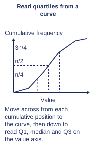
- Quartiles from curves — Locate n/4, n/2 and 3n/4 on the cumulative axis, move horizontally to the curve and down to the value axis. Read Q1, median and Q3; between recorded boundaries the result is an estimate. Label axes and retain enough graph precision for sensible readings.
Q1 is the lower quartile and Q3 is the upper quartile. Quartiles divide ordered data into four parts containing roughly equal numbers of observations.
- Box plots — Plot minimum, Q1, median, Q3 and maximum on a common numerical scale. The box shows the middle half; whiskers (lines extending from the box to the extremes) show the remaining range in an ordinary GCSE box plot. Equal widths of boxes are presentation, not frequencies; compare medians and IQRs in context.
IQR means interquartile range: Q3 − Q1, the spread of the middle half of the observations.
- Discrete cumulative data — For discrete observations a cumulative frequency gives counts at or below successive possible values; check the wording before reading below or at most. The display needs to respect possible values. For grouped continuous data readings inside intervals are estimates rather than exact recorded values.
Shape and skew
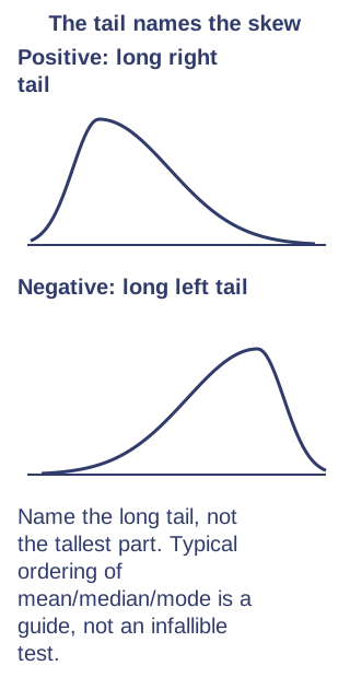
- Positive and negative skew — Positive skew has a longer tail towards large values; negative skew tails towards small values. The tail names the skew, not the location of the tallest bar. Typical positively skewed data have mean above median above mode, but inspect the full distribution rather than treating this as an infallible test.
- Box-plot evidence — A median closer to Q1 than Q3 suggests greater spread above the median and can support positive skew. Compare whiskers and the overall shape as well; a box plot hides detailed clusters, gaps and modes, so it cannot establish every distribution feature.
- Interpret shape — Explain where values concentrate and where unusual values occur, using the variable's context. A few large waiting times may pull the mean above most waits. Compare shape, centre and spread together; a higher median need not mean every observation is higher.
Higher — density and calculated skew
- Frequency density — For unequal-width histogram classes, density = frequency / class width. Bar area, not height alone, represents frequency. With frequency 12 in width 4 the density is 3; with frequency 20 in width 10 it is 2. The taller bar can therefore have fewer observations.
Unequal widths: area represents frequency. Original illustrative diagram; numerical datasets are fictional worked examples. Enlarge diagram - Recover histogram counts — Multiply density by class width to recover frequency. If a bar spans 20–30 at density 1.5, it represents 15 observations. A partial bar area estimates counts in a subinterval only if an even spread within that class is assumed.
- Skew coefficient — Use the supplied formula 3(mean − median) / standard deviation. With mean 24, median 22 and standard deviation 6, coefficient = 1, suggesting positive skew. It is dimensionless (it has no unit); zero does not alone prove a normal distribution, and zero standard deviation makes this formula undefined.
The example calculation is 3 × (24 − 22) ÷ 6 = 1.