 Mr Kidman's Classroom



Revise the key ideas
Preparing and calculating
- Original practice dataset — Fictional Harbour Pool data uses A1:D4 headings Session, Tickets, Price and Income. Rows 2–4 are Swim/12/5, Aqua/8/6 and Swim/10/5. Prices are pounds. These small invented records teach methods and are not a live Pearson dataset. Keep a Raw sheet, a Working sheet and a Dashboard so processing remains traceable.
A cell reference combines a column letter and row number: B2 is column B, row 2. Put the headings in row 1 and the three booking records in rows 2–4.
- Import and split — Import external CSV, workbook or suitable web data and check headings, delimiter, encoding and data types. Preview dates and numbers so text is not misread. Text to columns splits on a delimiter such as a comma or at fixed character widths; choose the method that matches the source. Check record counts and totals before relying on the import.
CSV means comma-separated values, a text format for tabular data. Encoding tells the software how to read characters; the wrong setting can turn symbols such as £ into incorrect characters.
- Arithmetic formulae — In D2 enter =B2*C2 to calculate £60, then fill down to obtain £48 and £50. Use +, -, * and / for addition, subtraction, multiplication and division; brackets control order. Revenue is quantity multiplied by price, whereas profit subtracts relevant costs. Currency formatting changes the display, not the underlying value.
- Summary functions — =SUM(D2:D4) gives 158; =AVERAGE(B2:B4) gives 10; =MIN(B2:B4) gives 8 and =MAX(B2:B4) gives 12. Select the intended range and explain what the statistic measures. AVERAGE usually ignores empty cells but includes zeros, so a missing value can change the interpretation. Independently check simple totals by hand.
- Cell references — Relative references adjust when a formula is copied. If F1 contains a 0.10 discount rate, =D2*(1-$F$1) gives 54 and can fill down while F1 stays fixed. $F$1 fixes both row and column; $F1 fixes the column and F$1 fixes the row. A named cell such as DiscountRate can make the same calculation easier to read.
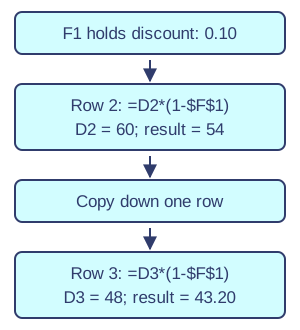
Copying a relative and absolute reference. Original illustration. Open full-size diagram - Sorting and filtering — Sort the whole table to preserve records; sort by Session and then Tickets to order within groups. Filtering hides nonmatching records without deleting them. Numeric criteria include greater than, less than and equals; text criteria include contains, begins with and ends with. Numbers stored as text can give unexpected ordering: check types first. For example, character-by-character ordering can place 10 before 2, unlike numeric ordering.
Conditional and lookup methods
- IF decisions — =IF(B2>=10,"Busy","Quiet") returns Busy for 12 tickets and Quiet for 8. The comparison is the logical test; text outputs use quotes. Test values below, exactly at and above the threshold so >= is not accidentally replaced by >. An IF labels a condition; it does not explain why demand changed.
- Logical operators — AND requires all conditions, OR requires at least one, and NOT reverses a logical result. =IF(AND(B2>=10,C2<=5),"Offer","Standard") gives Offer for row 2. Test combinations: 12 tickets at £6 fails the price condition. Brackets and clear tests matter more than memorising a long formula without understanding it.
- Conditional totals and counts — =SUMIF(A2:A4,"Swim",D2:D4) totals Swim income as 110. =COUNTIF(A2:A4,"Swim") counts two matching records, not 22 tickets. COUNTBLANK counts empty cells; COUNTA counts nonempty cells, including text and numbers. Keep criteria and sum ranges aligned. A formula returning an empty string can behave differently from a truly empty cell.
- Lookups — With H2:I3 holding Swim/5 and Aqua/6, =VLOOKUP(A2,$H$2:$I$3,2,FALSE) returns 5. It searches the first column and returns column 2 from the matched row. HLOOKUP searches the top row and returns from a specified row. Use exact matches for codes; check missing and duplicate keys and freeze the lookup table when copying.
- What-if modelling — What-if analysis changes assumptions and observes calculated outcomes; WHATIF names an approach here, not a universal spreadsheet function. Put a trial price in a separate input cell and link projected income to it. At 30 tickets, £5 gives £150 and £6 gives £180 only if quantity stays constant. Explain that higher prices might reduce demand.
Organisation and automation
- Grouping and subtotals — Group related rows or columns into an outline that can collapse and expand without deleting detail; ungroup restores the ungrouped view. Subtotals summarise groups using SUM, AVERAGE, MIN, MAX, COUNT or COUNTA. Sort records into the intended groups before inserting group subtotals. Choose whether hidden or filtered rows should contribute and check the tool's behaviour.
- Linked worksheets — Link a Dashboard cell to =Working!D5 rather than retyping a total. Separate raw data, calculations and presentation, label inputs and document assumptions with comments. Check references after renaming sheets or extending ranges. Multiple worksheets improve organisation only if links update correctly; a copied static figure can become stale.
For this example, first put =SUM(D2:D4) in cell D5 on the Working sheet. Then =Working!D5 on the Dashboard displays the linked total of 158.
- Views and display — Freeze panes to keep headings visible while scrolling. Hide or unhide irrelevant rows and columns for a task, but do not treat hiding as security. Comments explain assumptions without changing values. Conditional formatting uses data bars, colour scales or icons to show patterns; keep a legend and text or values so colour is not the only signal.
- Macros — A macro automates repeated steps, such as navigating to a dashboard or changing chart ranges or options. Plan the steps, use appropriate software support, test on a copy and check the final result. Do not enable an untrusted file's macros just to view its data. A recorded action may rely on a fixed selection and fail when rows change.
- Testing a workbook — Check arithmetic independently, test IF boundaries, missing lookup keys, empty cells, added rows and changing input values. Confirm charts, totals and controls update from linked data and that filters do not unexpectedly alter a calculation. Record expected and actual results. A workbook with no displayed error codes can still calculate the wrong measure.
Organisation and automation
- A complete summary — Using the existing Harbour Pool records, create a two-row summary with Swim and Aqua labels. Beside Swim, =SUMIF(Working!$A$2:$A$4,A2,Working!$B$2:$B$4) gives 22 tickets; copying down for Aqua gives 8. The dollar signs keep both source ranges fixed while A2 changes to A3. A column chart based on the summary should display 22 and 8, not three separate raw booking records. Change one ticket value, then check the formula and chart both update. New rows outside the range require an expanded range or an appropriately managed table.


