Types of data — Categorical data are labels such as transport mode. Discrete numerical data are countable values such as sibling count; continuous data such as height can take any value in an interval. Recorded rounding does not change the underlying type.
Questions and collection — Define the population, meaning the whole group you want to learn about, and the question before collecting data. A sample is the smaller group from which you collect observations. A sample may be biased if it excludes relevant groups or encourages a preferred answer. Fictional class data are examples, not evidence about a real school.
Frequency tables — Frequency counts how often a value or category occurs. For scores 1,2,3 with frequencies 2,5,3, there are 10 observations. A frequency is a count, not the data value itself.
Grouped data — For continuous lengths use non-overlapping intervals such as 0 ≤ x < 10, 10 ≤ x < 20. Grouping loses individual values; using each interval’s middle value to estimate its observations gives an estimated mean, not necessarily the exact mean.
Representations
Bar charts and line charts — Bar-chart heights show frequencies of categories or discrete values; gaps separate categories. A vertical line chart can show numerical values with a line at each value. Label axes and use an honest scale, usually starting a frequency axis at zero.
Pictograms — A key may state one symbol represents 4 pupils, so half a symbol represents 2. Multiply symbol counts by the key and show partial symbols consistently. Without the key the numerical interpretation is incomplete.
Pie charts — A sector angle is category frequency/total × 360°. If 12 of 40 pupils cycle, angle = 108°. Check all sectors sum to 360°; compare proportions rather than sector sizes across pies with different totals.
Grouped numerical charts — For equal-width intervals, a frequency bar chart can compare groups. Label intervals clearly and recognise that exact values within a bar are unknown. For unequal-width intervals, histogram bars need a different scale: their areas, rather than just their heights, represent frequencies. That method is a later extension; do not read unequal-width bars as simple frequency heights.
Misleading displays — Truncating a vertical axis can exaggerate a difference; changing symbol area rather than height may distort a pictogram. Read labels, scale, key, sample and source before accepting a visual claim.
Centre and spread
Mean — Add values and divide by the number of observations. For 2,4,4,10, mean = 20/4 = 5. From a table, sum value × frequency and divide by total frequency, not by the number of rows.
Median — Order values then find the middle. For 2,4,4,10 the median is (4 + 4)/2 = 4. For n observations the middle position is (n + 1)/2; an even n uses the mean of two middle values.
Mode — The mode is the most frequent value or category. Data can have multiple modes or no single mode. For grouped data the modal class is the interval with greatest frequency, not an exact modal value.
Range and outliers — Range = maximum − minimum. For 2,4,4,10 it is 8. An unusually high or low observation can strongly affect mean and range, while median may remain stable. Investigate rather than automatically delete an outlier.
Comparing distributions — Class A scores 4,5,6 and class B scores 1,5,9 have the same mean 5 but ranges 2 and 8. A has less spread. State both a centre and a spread in context; neither alone describes the full distribution.
Grouped estimates — For non-overlapping intervals 0 ≤ x < 10 and 10 ≤ x < 20 with frequencies 3 and 7, use midpoints 5 and 15: estimated mean = (3 × 5 + 7 × 15)/10 = 12. The true mean depends on the unknown values within the groups.
Relationships
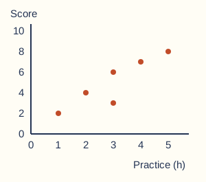
Scatter graphs — Plot each paired observation (x,y) once. An upward trend indicates positive correlation, a downward trend negative, and no clear trend suggests no correlation. The same x-value may have different y-values.Paired observations. Original illustrative model. Full-size diagram
Correlation and cause — A relationship between ice-cream sales and sunglasses sales may reflect sunny weather affecting both. Correlation alone does not establish that one variable causes the other. Observational data may contain confounding factors: other influences, such as sunny weather here, that help explain the relationship.
Predictions — A reasonable line of best fit follows the overall trend with points on both sides; it need not pass through the origin. Interpolation predicts inside the observed range; for example, predicting a value at x = 5 from data with x between 2 and 8. Extrapolation predicts outside that range, such as x = 20, and is less secure because the trend may change. A prediction is an estimate.
Experimental and observational — In an experiment a factor is deliberately changed while others are controlled where possible. In an observational study variables are recorded without that intervention. Both need careful sampling, measurement and cautious conclusions.
Enquiry
Evaluate a conclusion — State the question, graph or summary used, sample size, unusual values and limitations. A class survey cannot automatically represent all pupils nationally. Revisit the question after analysing rather than reporting only a calculated mean.
Test yourself
50 questions · Random sets of 10. These quick checks support revision; practise longer explanations and justified judgements too.
Mind map
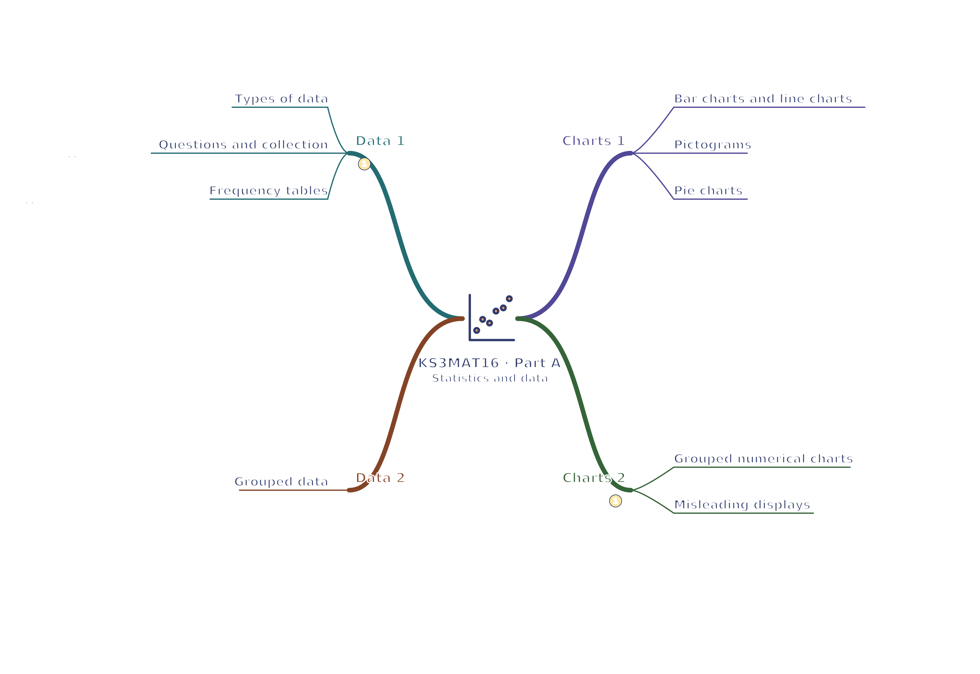
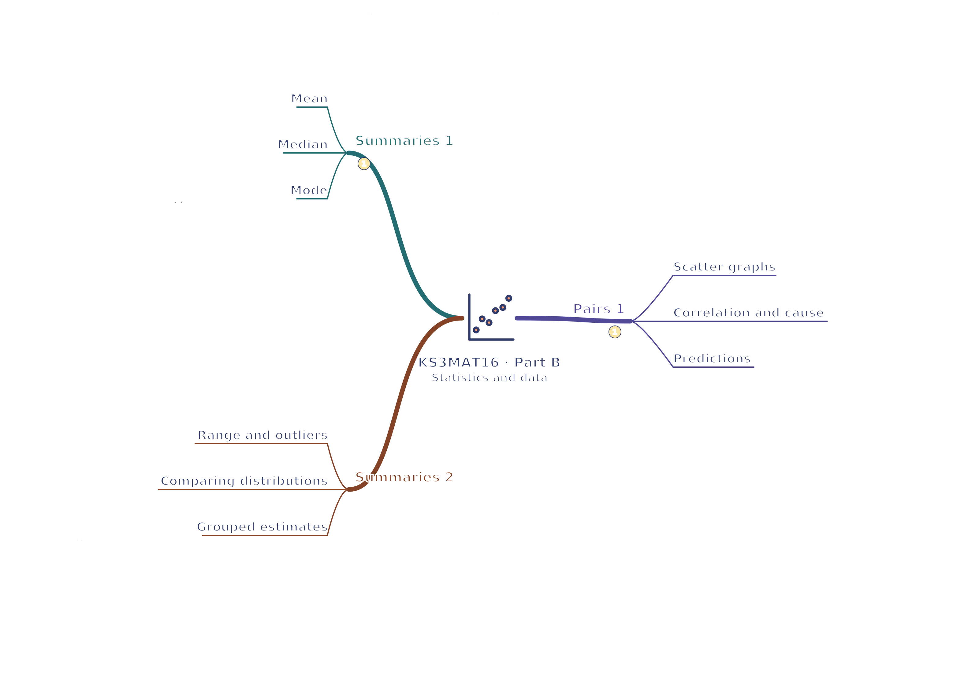
Use the branches to recall the ideas and explain their connections. Check the revision notes for the full detail.
KS3MAT16 · 1
View KS3MAT16 · 1 mind mapOpen the full-size map to zoom. Use the printable view for A4 landscape or enlarge to A3.
 Mr Kidman's Classroom